Survey

The survey is where everything comes together. It takes a scene, a scanner and a platform and the so-called “legs” that define the positions/trajectories of the platform during the survey and the speicifc settings of the scanner.

[1]:

import copy
import pandas as pd
import helios

Let’s demonstrate this for a basic ALS survey and prepare the platform, scanner and scene.

[2]:

platform = helios.platform_from_name("sr22")
scanner = helios.scanner_from_name("leica_als50")
sceneparts = helios.ScenePart.from_objs("../data/sceneparts/toyblocks/*.obj")
scene = helios.StaticScene(sceneparts)

From this, we can create an “empty” survey, which we can then populate with legs and settings:

[3]:

survey = helios.Survey(scene=scene, scanner=scanner, platform=platform)

[4]:

# no legs defined yet
survey.legs

[4]:

()

To use surveys created for ealier versions of helios (< v3.0.0), we can also load surveys from XML files. To make sure the survey can be loaded correctly, add the directory where the survey XML file is located as an asset directory (here: the root directory of the cloned helios repository):

[5]:

helios.add_asset_directory("D:/Software/_helios_versions/helios/")
tls_toyblocks_survey = helios.Survey.from_xml(
    "data/surveys/toyblocks/tls_toyblocks.xml"
)

Scanner settings

Scanner settings are defined per leg. Often, many or all legs of a survey will share the same scanner settings. We can define them once and then pass them to the legs. Depending on the optics of the respective scanner, different scan settings are relevant.

Note that we always specify the unit of the settings, resolving any ambiguity and ensuring that the settings are correctly interpreted. This is done by the help of the package pint. We can either specify the units by multiplying with the unit from helios.units or by using a string with the unit.

[6]:

scan_settings = helios.ScannerSettings(
    pulse_frequency=100_000 * helios.units.Hz,
    scan_angle=20 * helios.units.deg,
    scan_frequency="70 Hz",
    trajectory_time_interval=0.01 * helios.units.s,
)

Platform settings

Likewise, we also have platform settings. We can use PlatformSettings for static platforms and DynamicPlatformSettings for moving platforms. The latter allows us to specify the speed of the platform, or - if using interpolated trajectory, the trajectory settings. However, since platform settings are usually not shared between legs, we will often just specify the individual parameters directly when constructing or adding legs.

Legs

Legs are the positions or waypoints of a survey. In trajectory mode, they can also be portions of a given trajectory.

We define a list of waypoints that the airplane should fly through during the survey. Additionally, we set the speed of the platform.

[7]:

waypoints = [[-50, -25, 250], [50, -25, 250], [50, 25, 250], [-50, 25, 250]]
speed = 30  # m/s

Using a simple loop, we now add the legs at the respective positions and apply the scan settings.

[8]:

for x, y, z in waypoints:
    survey.add_leg(x=x, y=y, z=z, speed_m_s=speed, scanner_settings=scan_settings)

Running a survey

When running a survey, we can provide ExecutionSettings and OutputSettings to control the execution of the survey and the output format.

Execution settings

For example, we can explicitly change the number of threads, the logging verbosity or the parallelization strategy.

[9]:

execution_settings = helios.ExecutionSettings(
    num_threads=4,
    verbosity=helios.LogVerbosity.VERY_VERBOSE,
    parallelization=helios.ParallelizationStrategy.WAREHOUSE,
)

[10]:

pc, traj = survey.run(execution_settings=execution_settings)

Output settings

The output settings allow to change the format in which the output is returned (incl. requesting waveform and pulse output), the directory where the output is written (if written to file), and more. We show a few options below.

[11]:

# default
output_settings = helios.OutputSettings(format=helios.OutputFormat.NPY)
# return a laspy object
output_settings = helios.OutputSettings(format=helios.OutputFormat.LASPY)
# write to LAZ and change the las scale
output_settings = helios.OutputSettings(
    format=helios.OutputFormat.LAZ, las_scale=0.00025
)
# write to LAS and also write waveform and pulse output, use a custom output directory
output_settings = helios.OutputSettings(
    format=helios.OutputFormat.LAS,
    output_dir="detailed_output",
    write_waveform=True,
    write_pulse=True,
)
# write to XYZ and split by channel (relevant for multi-channel devices)
output_settings = helios.OutputSettings(
    format=helios.OutputFormat.XYZ, split_by_channel=True
)

Live view

When running a survey, we can also specify callbacks that are called during the survey execution. We use such callbacks for helios-live, which can be enables with live=True. This will show the virtual scene and the point collection in real time during the survey execution. The live view can be customized by providing a custom LiveViewer instance with specific settings.

pc, traj = survey.run(live=True, num_threads=1)

Output formats

Note that depending on the chosen output format, the survey.run() method has either one of two returns:

OutputFormat.NPY / OutputFormat.LASPY: two returns, a points array (or LASPY object) and a trajectory array
OutputFormat.LAS / OutputFormat.LAZ / OutputFormat.XYZ: one return, the path to the output folder

Below is a demonstration of the different output formats. Here you can also see that the individual parameters of ExecutionSettings and OutputSettings can be passed directly to the survey.run() method, without explicitly creating the settings objects.

[12]:

# output to arrays: returns two arrays
# numpy
pc, traj = survey.run(format=helios.OutputFormat.NPY)
# laspy
las, traj2 = survey.run(
    format=helios.OutputFormat.LASPY,
    parallelization=helios.ParallelizationStrategy.WAREHOUSE,
)

# output to file: returns one Path object (path to the output directory)
outpath_laz = survey.run(
    format=helios.OutputFormat.LAZ, verbosity=helios.LogVerbosity.VERY_VERBOSE
)

This is what the output looks like in each case:

OutputFormat.NPY

[13]:

# all simulated points and their attributes
pc[:10]

[13]:

array([(0, 1, [-24.2681    ,  17.55345567,   9.92294654], [-4.49147234e-13,  1.74036743e-01, -9.84739159e-01], [-61.073084 , -27.807459 , 230.4609125], 244.50845806, 6.62253898, 0., 1, 1, 919110, 0, 211257.85774, 0),
       (0, 1, [-24.2678    ,  17.52260986,   8.61144788], [-4.46472962e-13,  1.73000509e-01, -9.84921735e-01], [-61.072784 , -27.807459 , 230.4609125], 245.7947099 , 2.51876412, 0., 1, 1, 919111, 0, 211257.85775, 0),
       (0, 1, [-24.2675    ,  17.49266894,   7.27902349], [-4.43798194e-13,  1.71964083e-01, -9.85103220e-01], [-61.072484 , -27.807459 , 230.4609125], 247.10200063, 1.38474619, 0., 1, 1, 919112, 0, 211257.85776, 0),
       (0, 1, [-24.2672    ,  17.4956505 ,   5.74072633], [-4.41122936e-13,  1.70927467e-01, -9.85283615e-01], [-61.072184 , -27.807459 , 230.4609125], 248.61803247, 1.37794712, 0., 1, 1, 919113, 0, 211257.85777, 0),
       (0, 1, [-24.2669    ,  17.52363764,   4.03860207], [-4.38447189e-13,  1.69890661e-01, -9.85462918e-01], [-61.071884 , -27.807459 , 230.4609125], 250.30002994, 1.36743566, 0., 1, 1, 919114, 0, 211257.85778, 0),
       (0, 1, [-24.2666    ,  17.50822467,   2.56885104], [-4.35770957e-13,  1.68853668e-01, -9.85641131e-01], [-61.071584 , -27.807459 , 230.4609125], 251.74593591, 1.3572132 , 0., 1, 1, 919115, 0, 211257.85779, 0),
       (0, 1, [-24.2663    ,  17.51369089,   0.95831451], [-4.33094242e-13,  1.67816488e-01, -9.85818252e-01], [-61.071284 , -27.807459 , 230.4609125], 253.33441019, 1.34727307, 0., 1, 1, 919116, 0, 211257.8578 , 0),
       (0, 1, [-23.9555    ,  17.21470954,   5.83056158], [-4.38447189e-13,  1.69890661e-01, -9.85462918e-01], [-60.760484 , -27.807459 , 230.4609125], 248.48163629, 3.7578878 , 0., 1, 1, 920152, 0, 211257.86816, 0),
       (0, 1, [-23.9552    ,  17.2245571 ,   7.30340018], [-4.41122936e-13,  1.70927467e-01, -9.85283615e-01], [-60.760184 , -27.807459 , 230.4609125], 247.03201822, 3.81641334, 0., 1, 1, 920153, 0, 211257.86817, 0),
       (0, 1, [-23.9549    ,  17.19979667,   8.95675418], [-4.43798194e-13,  1.71964083e-01, -9.85103220e-01], [-60.759884 , -27.807459 , 230.4609125], 245.39889922, 3.84969181, 0., 1, 1, 920154, 0, 211257.86818, 0)],
      dtype=[('channel_id', '<u8'), ('hit_object_id', '<i4'), ('position', '<f8', (3,)), ('beam_direction', '<f8', (3,)), ('beam_origin', '<f8', (3,)), ('distance', '<f8'), ('intensity', '<f8'), ('echo_width', '<f8'), ('return_number', '<i4'), ('number_of_returns', '<i4'), ('fullwave_index', '<i4'), ('classification', '<i4'), ('gps_time', '<f8'), ('point_source_id', '<u2')])

[14]:

# only xyz position of simulated points
pc["position"][:10]

[14]:

array([[-24.2681    ,  17.55345567,   9.92294654],
       [-24.2678    ,  17.52260986,   8.61144788],
       [-24.2675    ,  17.49266894,   7.27902349],
       [-24.2672    ,  17.4956505 ,   5.74072633],
       [-24.2669    ,  17.52363764,   4.03860207],
       [-24.2666    ,  17.50822467,   2.56885104],
       [-24.2663    ,  17.51369089,   0.95831451],
       [-23.9555    ,  17.21470954,   5.83056158],
       [-23.9552    ,  17.2245571 ,   7.30340018],
       [-23.9549    ,  17.19979667,   8.95675418]])

[15]:

# trajectory
traj[:10]

[15]:

array([(211257.  , [-50.0003, -25.    , 250.    ], -0., 0., 4.71238898),
       (211257.01, [-49.7003, -25.    , 250.    ], -0., 0., 4.71238898),
       (211257.02, [-49.4003, -25.    , 250.    ], -0., 0., 4.71238898),
       (211257.03, [-49.1003, -25.    , 250.    ], -0., 0., 4.71238898),
       (211257.04, [-48.8003, -25.    , 250.    ], -0., 0., 4.71238898),
       (211257.05, [-48.5003, -25.    , 250.    ], -0., 0., 4.71238898),
       (211257.06, [-48.2003, -25.    , 250.    ], -0., 0., 4.71238898),
       (211257.07, [-47.9003, -25.    , 250.    ], -0., 0., 4.71238898),
       (211257.08, [-47.6003, -25.    , 250.    ], -0., 0., 4.71238898),
       (211257.09, [-47.3003, -25.    , 250.    ], -0., 0., 4.71238898)],
      dtype=[('gps_time', '<f8'), ('position', '<f8', (3,)), ('roll', '<f8'), ('pitch', '<f8'), ('yaw', '<f8')])

OutputFormat.LASPY

[16]:

print(las)
print(las.x)
print(las.gps_time)

<LasData(1.4, point fmt: <PointFormat(6, 12 bytes of extra dims)>, 43847 points, 1 vlrs)>
<ScaledArrayView([-24.2  -24.2  -24.2  ...   2.43   2.43   2.43])>
[211257.86001 211257.86002 211257.86003 ... 211263.58571 211263.58572
 211263.58573]

[17]:

# the trajectory output is the same in both NPY and LASPY cases
traj2[:10]

[17]:

array([(211257.  , [-50.0003, -25.    , 250.    ], 0., 0., 4.71238898),
       (211257.01, [-49.7003, -25.    , 250.    ], 0., 0., 4.71238898),
       (211257.02, [-49.4003, -25.    , 250.    ], 0., 0., 4.71238898),
       (211257.03, [-49.1003, -25.    , 250.    ], 0., 0., 4.71238898),
       (211257.04, [-48.8003, -25.    , 250.    ], 0., 0., 4.71238898),
       (211257.05, [-48.5003, -25.    , 250.    ], 0., 0., 4.71238898),
       (211257.06, [-48.2003, -25.    , 250.    ], 0., 0., 4.71238898),
       (211257.07, [-47.9003, -25.    , 250.    ], 0., 0., 4.71238898),
       (211257.08, [-47.6003, -25.    , 250.    ], 0., 0., 4.71238898),
       (211257.09, [-47.3003, -25.    , 250.    ], 0., 0., 4.71238898)],
      dtype=[('gps_time', '<f8'), ('position', '<f8', (3,)), ('roll', '<f8'), ('pitch', '<f8'), ('yaw', '<f8')])

OutputFormat.LAZ (output to file)

[18]:

outpath_laz

[18]:

WindowsPath('d:/Software/_helios_versions/helios/doc/output/2026-05-26_12-41-11')

Running multiple surveys

In practice, we often need to run multiple surveys to create different dataset variations, e.g., using different scanner settings, trajectories, or scenes. Rather than loading these components again for each survey, we can reuse them. Currently, when reusing the same scanner, platform, or scene objects across multiple surveys, they need to be deep-copied as demonstrated below to avoid a ValueError. The reason is that with the current design of helios, reusing them without copying would couple their internal states in unforeseen and unintended ways.

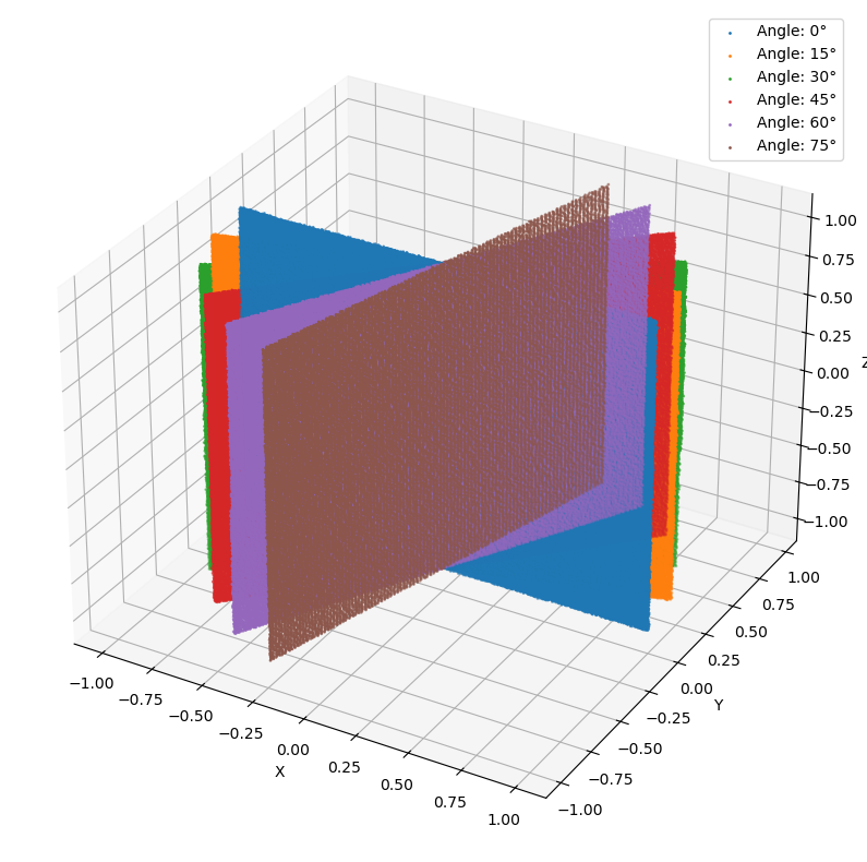
Example 1: Modifications of the scene

[19]:

scanner = helios.scanner_from_name("riegl_vz_600i")
platform = helios.platform_from_name("tripod")
plane = helios.ScenePart.from_obj("../data/sceneparts/basic/plane/plane.obj").rotate(
    axis=(1, 0, 0), angle=90 * helios.units.deg
)
x, y, z = [0, -10, 0]
scanner_settings = helios.ScannerSettings(
    pulse_frequency=1_200_000 * helios.units.Hz,
    horizontal_resolution=0.03 * helios.units.deg,
    vertical_resolution=0.03 * helios.units.deg,
    rotation_start_angle=-20 * helios.units.deg,
    rotation_stop_angle=20 * helios.units.deg,
    trajectory_time_interval=0.01 * helios.units.s,
)

results = {}
for angle in range(0, 90, 15):
    print(f"Running survey with plane rotated by {angle} degrees around the z-axis...")
    survey = helios.Survey(
        scene=helios.StaticScene(
            [
                copy.deepcopy(plane).rotate(
                    axis=(0, 0, 1), angle=angle * helios.units.deg
                )
            ]
        ),
        scanner=copy.deepcopy(scanner),
        platform=copy.deepcopy(platform),
    )
    survey.add_leg(x=x, y=y, z=z, scanner_settings=scanner_settings)
    pc, _ = survey.run(format=helios.OutputFormat.NPY)
    results[angle] = pc["position"]

Running survey with plane rotated by 0 degrees around the z-axis...

Running survey with plane rotated by 15 degrees around the z-axis...

Running survey with plane rotated by 30 degrees around the z-axis...

Running survey with plane rotated by 45 degrees around the z-axis...

Running survey with plane rotated by 60 degrees around the z-axis...

Running survey with plane rotated by 75 degrees around the z-axis...

[20]:

# Display the results with matplotlib
import matplotlib.pyplot as plt

# 3d figure
fig = plt.figure(figsize=(10, 10))
ax = fig.add_subplot(111, projection="3d")
for i, (angle, pc) in enumerate(results.items()):
    ax.scatter(pc[:, 0], pc[:, 1], pc[:, 2], s=1, label=f"Angle: {angle}°")
ax.set_xlabel("X")
ax.set_ylabel("Y")
ax.set_zlabel("Z")
plt.legend()
plt.show()

Example 2: Modifications of full waveform settings

To test different full waveform settings for the same scene, we use the utility function combine_parameters. To create the parameter combinations, we change the bin_size, win_size, and beam_sample_quality variables. The combine_parameters function is documented in detail in the Utility functions section, and more information on the full waveform is provided in the Full waveform and intensity modelling section.

[21]:

# full waveform parameters to be tested
bin_sizes = [0.25, 0.1, 0.05]  # discretization of the waveform in time (ns)
win_sizes = [2, 1, 0.5]  # pulse length (ns)
beam_sample_qualities = [
    3,
    5,
]  # number of concentric circles of subrays for discretization in space

scanner = helios.scanner_from_name("riegl_vux_1uav")
platform = helios.platform_from_name("copter_linearpath")
scanner_settings = helios.ScannerSettings(
    pulse_frequency=300_000 * helios.units.Hz,
    scan_frequency=60 * helios.units.Hz,
    trajectory_time_interval=0.01 * helios.units.s,
)

tree1 = helios.ScenePart.from_obj(
    "../data/sceneparts/arbaro/sassafras_low.obj", up_axis="y"
)
groundplane = helios.ScenePart.from_obj(
    "../data/sceneparts/basic/plane/plane.obj"
).scale(20)
scene = helios.StaticScene([groundplane, tree1])

return_metric_results = {}
# combine parameters for fwfsettings
for params in helios.combine_parameters(
    bin_size=bin_sizes, win_size=win_sizes, beam_sample_quality=beam_sample_qualities
):
    fwf_settings = helios.FullWaveformSettings(
        bin_size=params["bin_size"] * helios.units.ns,
        win_size=params["win_size"] * helios.units.ns,
        beam_sample_quality=params["beam_sample_quality"],
    )
    # make sure to use deepcopy on all the assets that are used in multiple runs
    survey = helios.Survey(
        scene=copy.deepcopy(scene),
        scanner=copy.deepcopy(scanner),
        platform=copy.deepcopy(platform),
        full_waveform_settings=fwf_settings,
    )
    survey.add_leg(x=-10, y=0, z=50, speed_m_s=6, scanner_settings=scanner_settings)
    survey.add_leg(
        x=20, y=0, z=50, speed_m_s=6, scanner_settings=scanner_settings, is_active=False
    )
    pc, traj = survey.run(format=helios.OutputFormat.NPY)

    # compute return metrics and store in dict. This will allow the comparison of the returns from different settings.
    num_points = pc.shape[0]
    num_first_returns = (pc["return_number"] == 1).sum()
    num_multiple_returns = (pc["return_number"] > 1).sum()
    num_intermediate_returns = (
        (pc["return_number"] > 1) & (pc["return_number"] < pc["number_of_returns"])
    ).sum()
    ratio_intermediate = num_intermediate_returns / num_points
    ratio_multiple = num_multiple_returns / num_points
    return_metric_results[
        params["bin_size"], params["win_size"], params["beam_sample_quality"]
    ] = {
        "num_points": num_points,
        "num_first_returns": num_first_returns,
        "num_multiple_returns": num_multiple_returns,
        "ratio_multiple": ratio_multiple,
        "num_intermediate_returns": num_intermediate_returns,
        "ratio_intermediate": ratio_intermediate,
    }

Now we create a table to compare the return metrics for the different settings.

[22]:

return_df = pd.DataFrame.from_dict(
    return_metric_results,
    orient="index",
    columns=[
        "num_points",
        "num_first_returns",
        "num_multiple_returns",
        "ratio_multiple",
        "num_intermediate_returns",
        "ratio_intermediate",
    ],
)
return_df.index.names = ["bin_size", "win_size", "beam_sample_quality"]
# formatting
for k in return_df.keys():
    if "ratio" in k:
        return_df[k] = return_df[k].map(lambda x: f"{x:.3%}")
    elif "number" in k:
        return_df[k] = return_df[k].map(lambda x: f"{int(x):,}")

display(return_df)

			num_points	num_first_returns	num_multiple_returns	ratio_multiple	num_intermediate_returns	ratio_intermediate
bin_size	win_size	beam_sample_quality
0.25	2.0	3	180758	180001	757	0.419%	8	0.004%
	2.0	5	180975	180001	974	0.538%	22	0.012%
	1.0	3	186568	180001	6567	3.520%	663	0.355%
	1.0	5	187995	180001	7994	4.252%	983	0.523%
	0.5	3	187299	180001	7298	3.896%	905	0.483%
	0.5	5	188885	180001	8884	4.703%	1299	0.688%
0.10	2.0	3	180820	180001	819	0.453%	8	0.004%
	2.0	5	181028	180001	1027	0.567%	20	0.011%
	1.0	3	186686	180001	6685	3.581%	678	0.363%
	1.0	5	188101	180001	8100	4.306%	988	0.525%
	0.5	3	187371	180001	7370	3.933%	880	0.470%
	0.5	5	188946	180001	8945	4.734%	1262	0.668%
0.05	2.0	3	180755	180001	754	0.417%	8	0.004%
	2.0	5	180953	180001	952	0.526%	19	0.010%
	1.0	3	186544	180001	6543	3.507%	655	0.351%
	1.0	5	187939	180001	7938	4.224%	949	0.505%
	0.5	3	187211	180001	7210	3.851%	816	0.436%
	0.5	5	188746	180001	8745	4.633%	1180	0.625%

We can observe the following trends in the results:

We usually get more points and multiple returns with higher beam sample quality since sampling more subrays within the footprint increases the chances of registering multiple returns.
The number of multiple returns also increases with smaller window sizes. The window size is used in the maximum detection, so if the window size is smaller than the spacing between two returns, they can be registered as separate returns, leading to more multiple returns.

By comparing these numbers with a real-world reference, we may choose the full waveform settings that are most suitable for our simulation scenario.