TLS Risley Prism Scanner

Notebook: Hannah Weiser, 2026

This demo notebook demonstrates a terrestial laser scanning (TLS) survey with a risley beam deflector. This scanning technology results a non-repetitive, retina-like scan pattern, which means the point density depends on the integration time.

import helios
import numpy as np
import matplotlib.pyplot as plt

Virtual scene

We use the box scene, which is perfect for demonstrating the non-repetitive scan pattern of a risley beam deflector on a vertical wall.

box = helios.ScenePart.from_obj("../data/sceneparts/basic/box/box100.obj")
scene = helios.StaticScene([box])

Scanner and platform

We are simulating a Livox Mid-40 scanner and a Livox Mid-100 scanner, both mounted on a tripod. For this deflector type, the scan pattern is controlled by the rotation speeds (rotorFreq1_Hz and rotorFreq2_Hz), wedge angles (angle1_deg and angle2_deg) and refractive indices (refrIndex1 and refrIndex2) of two rotating risley prisms. The design on which the low-cost Livox scanners are based is described in detail in Liu et al. (2022). More information on the Livox sensors and their point cloud characteristics can be obtained from the Livox Wiki. For further reading on rotational risley prisms, see Duma & Schitea (2018).

scanner_mid40 = helios.scanner_from_name("livox_mid40")
scanner_mid100 = helios.scanner_from_name("livox_mid100")
platform = helios.platform_from_name("tripod")

Scan positions

To demonstrate influence of integration times on point density, we simulate three scan positions with integration times of 0.01 s, 0.1 s and 1 s.

survey_mid40 = helios.Survey(scene=scene, scanner=scanner_mid40, platform=platform)
survey_mid100 = helios.Survey(scene=scene, scanner=scanner_mid100, platform=platform)
x = y = z = 0.0
for survey in [survey_mid40, survey_mid100]:
    survey.add_leg(x=x, y=y, z=z, max_duration=0.01 * helios.units.s)
    survey.add_leg(x=x, y=y, z=z, max_duration=0.1 * helios.units.s)
    survey.add_leg(x=x, y=y, z=z, max_duration=1.0 * helios.units.s)

Running the survey

points_mid40, trajectories_mid40 = survey_mid40.run(
    verbosity=helios.LogVerbosity.VERBOSE, format=helios.OutputFormat.NPY
)
points_mid100, trajectories_mid100 = survey_mid100.run(
    verbosity=helios.LogVerbosity.VERBOSE, format=helios.OutputFormat.NPY
)

Visualizing the results

fig, axs = plt.subplots(2, 3, figsize=(16, 5), sharex=True, sharey=True)

for i, (points, scanner) in enumerate(
    zip([points_mid40, points_mid100], ["Livox Mid-40", "Livox Mid-100"])
):
    coords = points["position"]
    leg1 = points["point_source_id"] == 0
    leg2 = points["point_source_id"] == 1
    leg3 = points["point_source_id"] == 2

    axs[i, 0].scatter(
        coords[leg1, 0], coords[leg1, 2], s=0.01, c=points["gps_time"][leg1]
    )
    axs[i, 1].scatter(
        coords[leg2, 0], coords[leg2, 2], s=0.01, c=points["gps_time"][leg2]
    )
    axs[i, 2].scatter(
        coords[leg3, 0], coords[leg3, 2], s=0.01, c=points["gps_time"][leg3]
    )
    axs[i, 0].set_title(f"{scanner} - Integration time: 0.01 s")
    axs[i, 1].set_title(f"{scanner} - Integration time: 0.1 s")
    axs[i, 2].set_title(f"{scanner} - Integration time: 1.0 s")

for ax in axs.flat:
    ax.set_xlabel("X")
    ax.set_ylabel("Z")
    ax.set_aspect("equal", "box")

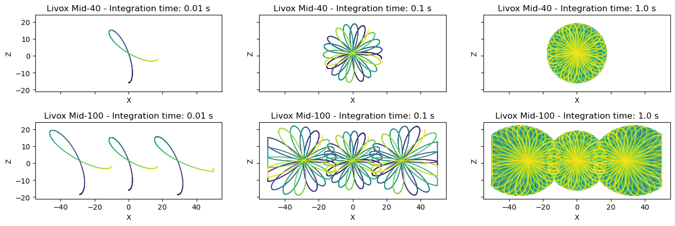
As stated in Liu et al. (2022), the scanning mechanisms results in a retina-like, non-repetitive scanning pattern, with the highest point density in the centre of the field of view. With increasing integration time, the point density increases. This is different for other deflector types, such as rotating mirrors, where the scanner itself needs to move or rotate in order to result in a nonrepeating pattern. For the Livox Mid-100, the “three-in-one version of Livox Mid-40” (Livox Mid-100 Quick Start Guide), the field of views of the three LiDAR sensors overlap, resulting in a wide horizontal field of view.