Scenes and scene parts

A scene is a collection of one or more scene parts. These are 3D models that can be loaded as triangle meshes or voxels.

import helios

Loading scene parts

Scene parts can be loaded with various input formats, including:

1. from OBJ files (for meshes)

2. from GeoTIFF files (for digital elevation models)

3. from XYZ point cloud files (for voxel models from point clouds)

4. from .vox voxel files (for voxel-based vegetation modelling)

5. from open3d geometries (for meshes or voxel models from point cloud)

1) OBJ files

For OBJ files, you only need to provide the path to the file. If material files are referenced in the OBJ files, the material properties will also be loaded. Alternatively, users can use the Material class to specify and modify material properties. Since OBJ files can have different orientations, i.e. different definitions of the “up axis”, you can specify the up axis when loading the file. By default, helios assumes that the up axis is “z”.

groundplane = helios.ScenePart.from_obj(
    "../data/sceneparts/basic/groundplane/groundplane.obj"
)
tree = helios.ScenePart.from_obj(
    "../data/sceneparts/arbaro/sassafras_low.obj", up_axis="y"
)  # Y as up-axis
type(tree)

helios.scene.ScenePart

2) TIFF files

Digital elevation models (DEMs) can be loaded as GeoTIFF files.

dem = helios.ScenePart.from_tiff("../data/sceneparts/tiff/dem_hd.tif")

HELIOS will use their encoded georeferencing information and resolution and build a triangle mesh. The centers of the pixels are used as data points. If all points are valid (following the invalid/NoData value definition from the GeoTIFF header), two triangles are built up: Current point - right neighbor - upper right neighbor and current point - upper neighbor - upper right neighbor:

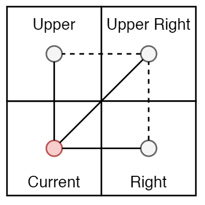
If any of the three points has an invalid value, the triangle is omitted.

3) XYZ files

helios can also load xyz point clouds as scene parts, transforming them into grids of cubic cells (“voxels”). If a cell contains at least one point, the cell is defined as “solid” and an axis-aligned bounding box primitive with the extent of the cell is created, providing a surface to be virtually scanned.

sphere = helios.ScenePart.from_xyz(
    "../data/sceneparts/pointclouds/sphere_dens25000.xyz", voxel_size=0.1
)

helios expects the columns in the file to have the following format: X Y Z Nx Ny Nz, where Nx Ny Nz are the optional normal vector components. The desired side length of a voxel is specified with the parameter voxel_size, controlling the level of detail of the voxel model.

To obtain ray incidence angles for voxels for the calculation of return intensity, different options are provided by helios. If the point cloud does not contain point normals, normals will always be calculated using Singular Value Decomposition (SVD). This is also possible if the point cloud contains normals by explicitly setting estimate_normals=True. For voxels containing less than three points, no normal can be estimated. These voxels are either discarded or they are assigned a default_normal if it is specified as a vector like this: default_normal=[0, 0, 1].

The default behaviour for point clouds with normals is to average the normals of each point within the voxel to derive the voxel normal. As an alternative, the normal of the point closest to the voxel center can be assigned as point normal by setting snap_neighbor_normal=True.

sphere = helios.ScenePart.from_xyz(
    "../data/sceneparts/pointclouds/sphere_dens25000.xyz",
    separator=" ",
    voxel_size=1.0,
    estimate_normals=True,
    default_normal=[0, 0, 1],
    snap_neighbor_normal=True,
)

4) VOX files

helios can read voxel models provided in a text format with .vox extension, inspired by the format used in the software AMAPVox software (Vincent et al. 2017). The primary purpose of this loader is to model vegetation with given leaf properties.

The content of a .vox file looks like this:

VOXEL SPACE
#min_corner: 12.464750289916992 -10.332499504089355 243.5574951171875
#max_corner: 21.312000274658203 -1.6010000705718994 272.84124755859375
#split: 36 35 118
#res:0.25 #nsubvoxel:8 #nrecordmax:0 #fraction-digits:7 #lad_type:Spherical #type:TLS #max_pad:5.0 #build-version:1.4.3
i j k PadBVTotal angleMean bsEntering bsIntercepted bsPotential ground_distance lMeanTotal lgTotal nbEchos nbSampling transmittance attenuation attenuationBiasCorrection
0 0 0 0 86.3137164 0.4989009 0 2.8475497 0.1240837 0.1632028 693.775004 0 4251 1 0 0
0 0 1 0 86.989336 1.011544 0 2.840831 0.3722511 0.1784628 1292.784752 0 7244 1 0 0
0 0 2 0 87.2224845 1.1786434 0 2.835464 0.6204185 0.1828753 1434.1079874 0 7842 1 0 0
0 0 3 0 87.1534196 0.9608315 0 2.8170681 0.8685859 0.1816032 1186.2322972 0 6532 1 0 0
0 0 4 0 87.2968587 0.8746295 0 2.8187793 1.1167532 0.1841085 1201.8604542 0 6528 1 0 0
0 0 5 0 87.1479655 0.9425028 0 2.8363264 1.3649206 0.1747828 1195.6891804 0 6841 1 0 0

The file (as of version 1.4.3) uses space as separator and has six header lines.

• Lines 2 and 3 define the axis aligned bounding box with the xyz coordinates of the minimum and maximum corners (#min_corner and #max_corner).

• Line 4 gives the number of voxels in x, y and z direction (#split).

• Line 5 defines the resolution (#res), the leaf angle distribution type (#lad_type) and the maximum plant area density value (#max_pad). It can furthermore contain additional information which are not read by HELIOS++.

• Line 6 contains the column names. The following are relevant for HELIOS++:

  • i, j, k: The voxel indices in x, y and z direction.

  • PADBVTotal is the plant area density (m2/m3). This parameter is used by HELIOS++ in the transmittive mode to calculate the return and in the scaled mode to determine the size of each voxel (see next sections)

More in-depth explanations are given in the AMAPVox 1.0.1 user guide (page 28) and in the AMAPVox GUI tooltips.

All following lines contain the voxel values with each line representing one voxel. Empty voxels (PADBVTotal = 0 and transmittance = 1) may or may not be explicitly defined.

There are three modes available for handling ray intersections with DetailedVoxels.

Transmittive mode (default)

transmittive_canopy = helios.ScenePart.from_vox(
    "../data/sceneparts/syssifoss/F_BR08_08_merged.vox",
    intersection_mode="transmittive",
)

In transmittive mode, voxels are considered to be filled with transmittive turbid medium. Each voxel is filled with randomly distributed infinitely small sized leaf scatterers. Voxels are therefore defined by a leaf area density (\(\mu_L\)) and a leaf angle distribution (\(g_L\)), from which the extinction coefficient \(\sigma\) is calculated (North 1996).

\[\sigma = \frac{\mu_L}{2\pi} \int_0^{2\pi} g_L \left| \Omega' \cdot \Omega_L \right| d\Omega_L\]

where \(\Omega'\) is the unit direction vector of the photon path and \(\Omega_L\) is the leaf normal vector.

If a ray intersects a voxel, the distance before collision \(s\) within the voxel is simulated from a random number \(R\) with uniform distribution in the range \((0 < R < 1)\) (North 1996):

\[s = \frac{-\ln (R)}{\sigma}\]

If the distance \(s\) is larger than the \(intersectionLength\), the ray continues through the voxel without generating a return (and may create a return when intersecting another geometry later on). If \(s\) is smaller than the \(intersectionLength\), the return within the voxel is calculated as:

\[IntersectionPoint = EntryPoint + s \cdot rayDirection\]

transmittive_canopy = helios.ScenePart.from_vox(
    "../data/sceneparts/syssifoss/F_BR08_08_merged.vox"
)  # since it is the default
# specifying the LAD LUT
transmittive_canopy = helios.ScenePart.from_vox(
    "../data/sceneparts/syssifoss/F_BR08_08_merged.vox",
    intersection_mode="transmittive",
    ladlut_path="../data/lut/spherical.txt",
)

Scaled mode

voxel_canopy_with_gaps = helios.ScenePart.from_vox(
    "../data/sceneparts/syssifoss/F_BR08_08_merged.vox",
    intersection_mode="scaled",
    intersection_argument=0.3334,
)

In scaled mode, each voxel is considered to be solid (non-transmittive) and of a specific size determined by the leaf area density according to the equation (adapted from AMAPVox OBJ export tool):

\[voxelSize= voxelResolution \cdot \left( \frac{pad}{pad_{max}} \right)^\alpha\]

where \(voxelResolution\) and \(pad_{max}\) are defined in header line 5, \(pad\) is the value read from the column PADBVTotal and \(\alpha\) is a scaling factor that is defined using the intersection_argument (default: 0.5). If a ray intersects a scaled voxel, the intersection point is returned.

There is also the option to shift voxels randomly within the original voxel resolution to disrupt the regular pattern of the voxels and to achieve more “natural” models using the boolean random_shift parameter.

voxel_canopy_with_gaps = helios.ScenePart.from_vox(
    "../data/sceneparts/syssifoss/F_BR08_08_merged.vox",
    intersection_mode="scaled",
    intersection_argument=0.3334,
    random_shift=True,
)

Fixed mode

voxel_canopy_25cm = helios.ScenePart.from_vox(
    "../data/sceneparts/syssifoss/F_BR08_08_crown_250.vox", intersection_mode="fixed"
)

In fixed mode, each voxel is modelled as solid (not light-transmittive) and of the size given by #res. Only Voxels with transmittance < 1 are considered to be filled. If a ray intersects a filled voxel, the intersection point on the surface is returned.

5) Open3D Geometries

helios provides an interface to open3d for loading both meshes and point clouds. If a mesh is provided, it is loaded as a triangle mesh similar to the OBJ loading. If a point cloud is provided, it is loaded as a voxel model similar to the XYZ loading. The same parameters are available for controlling the normal estimation and handling of voxels with less than three points as described in the XYZ section above.

This interface allows to load, build or manipulate 3D geometries with the powerful open3d library and then use them as scene parts in helios.

import open3d as o3d

# Loading an open3d mesh
monkey = o3d.data.MonkeyModel()
model = o3d.io.read_triangle_mesh(monkey.path)

monkey_scene_part = helios.ScenePart.from_open3d(model, up_axis="z")

Jupyter environment detected. Enabling Open3D WebVisualizer.
[Open3D INFO] WebRTC GUI backend enabled.
[Open3D INFO] WebRTCWindowSystem: HTTP handshake server disabled.

# Loading an open3d point cloud
pcd = o3d.io.read_point_cloud(
    "../data/sceneparts/pointclouds/sphere_dens25000_normals.xyz", format="xyzn"
)
pcd.crop(
    o3d.geometry.AxisAlignedBoundingBox(
        min_bound=(57.8, 14.8, 4.0), max_bound=(77.8, 34.8, 44.1)
    )
)  # cropping the sphere by half
cropped_sphere = helios.ScenePart.from_open3d(
    pcd, voxel_size=0.2, estimate_normals=False, snap_neighbor_normal=False
)

Loading multiple scene parts at one

Of course, these methods can be put into a loop to load a large number of scene parts at once. However, helios also supports loading multiple scene parts by specifying a path with wildcards to the respective from_objs, from_tiffs and from_xyzs methods. For example, if you have a folder with multiple OBJ files, you can load them all at once like this:

toyblocks = helios.ScenePart.from_objs("../data/sceneparts/toyblocks/*.obj")
type(toyblocks)

list

Transforming scene parts

Coordinate transformations can be applied to scene parts. This includes translations, rotations and scaling.

toyblock = helios.ScenePart.from_obj("../data/sceneparts/toyblocks/cube.obj")

1) Translate

To translate a scene part, simply provide the translation vector to the translate method:

toyblock.translate([5, 5, 0])
# or directly when loading the scene part:
toyblock = helios.ScenePart.from_obj("../data/sceneparts/toyblocks/cube.obj").translate(
    [5, 5, 0]
)

2) Rotate

To rotate a scene part, three rotation definitions are supported:

• Quaternion: Provide the four components of the quaternion as a list or array in the order [w, x, y, z].

• Axis-angle: Provide the rotation axis as a vector and the scalar rotation angle in degrees or radians.

• Vector-to-vector: Provide two vectors u and v and obtain the rotation of minimal angle that maps u to v.

In addition, a rotation_center can be specified to define the center of rotation. By default, the origin of the object is used as rotation center.

# same rotation for each definition
toyblock.rotate(
    axis=[0, 1, 0], angle=45 * helios.units.degree
)  # example for axis-angle rotation
toyblock.rotate(
    quaternion=[0.9238795, 0, 0.3826834, 0]
)  # example for quaternion rotation
toyblock.rotate(
    from_axis=[0, 0, 1], to_axis=[0.7071, 0, 0.7071]
)  # example for vector-to-vector rotation

<ScenePart at 0x1eadca0d6b0>

3) Scale

A scene part can be scaled by providing a scaling factor. Scaling will be applied uniformly in all directions. Non-uniform scaling is currently not supported. For non-uniform scaling, edit the scene part in external software, e.g. in Blender for mesh models.

toyblock.scale(2.0)

<ScenePart at 0x1eadca0d6b0>

Transformations can also be chained together and will then be applied in the order specified, which is especially relevant when not rotating around the object origin. This means that the following coordinate transformations are not equivalent.

toyblock1 = (
    helios.ScenePart.from_obj("../data/sceneparts/toyblocks/cube.obj")
    .translate([5, 5, 0])
    .rotate(
        axis=[0, 1, 0], angle=45 * helios.units.degree, rotation_center=[0.0, 0.0, 0.0]
    )
    .scale(2.0)
)
toyblock2 = (
    helios.ScenePart.from_obj("../data/sceneparts/toyblocks/cube.obj")
    .scale(2.0)
    .rotate(
        axis=[0, 1, 0], angle=45 * helios.units.degree, rotation_center=[0.0, 0.0, 0.0]
    )
    .translate([5, 5, 0])
)

We can see this by investigating their bounding boxes:

toyblock1.bbox.bounds

((47.807548872992086, -88.400208, -76.74523769795861),
 (104.49799233435176, -48.227797999999986, -20.05477868024975))

toyblock2.bbox.bounds

((45.73648106112661, -93.400208, -69.67416988609314),
 (102.42692452248629, -53.227797999999986, -12.983710868384271))

Creating, saving and loading scenes

A static scene can simply created from a list of scene parts. Scene parts can also be added to an existing scene via the add_scene_part method.

groundplane = helios.ScenePart.from_obj(
    "../data/sceneparts/basic/groundplane/groundplane.obj"
)
tree1 = helios.ScenePart.from_obj(
    "../data/sceneparts/arbaro/sassafras_low.obj", up_axis="y"
)
tree2 = helios.ScenePart.from_obj(
    "../data/sceneparts/arbaro/black_tupelo_low.obj", up_axis="y"
).translate([10, 0, 0])
scene = helios.StaticScene(scene_parts=[groundplane, tree1])
scene.add_scene_part(tree2)

Once created, a scene can be saved to a binary file and later loaded again from the binary file.

scene.to_binary("../arbaro_binary.bin")

loaded_scene = helios.StaticScene.from_binary("../arbaro_binary.bin")

A scene can also be loaded from an XML file. Here, it might be necessary to add an asset directory to the helios search path so that relative paths to the scene parts can be resolved.

helios.add_asset_directory("../")
scene = helios.StaticScene.from_xml("../data/scenes/demo/arbaro_demo.xml")

Bounding boxes

It can be useful to retrieve the axis-aligned bounding box of individual scene parts.

print(tree1.bbox.bounds)
print(tree1.bbox.centroid)

((-13.885534999999999, -9.00227, -13.945395), (4.061035, 8.3117, 10.405725000000002))
[-4.91225  -0.345285 -1.769835]

This is also possible for the whole scene:

print(scene.bbox.bounds)
print(scene.bbox.centroid)

((-100.0, -100.0, -6.9726975), (100.0, 100.0, 6.9726975))
[0. 0. 0.]

Material properties

Reading and modifying material properties of scene parts

Scene parts also have material properties, which we can access and modify. Let’s start with an example where the scene part already has a material.

material_names = list(tree1.materials.keys())

material_names

['trunk', 'stems_1', 'stems_2', 'stems_3', 'leaves']

print(tree1.materials["trunk"].spectra)
print(tree1.materials["trunk"].reflectance)
print(tree1.materials["trunk"].classification)
print(tree1.materials["trunk"].specular_components)
print(tree1.materials["trunk"].diffuse_components)
print(tree1.materials["trunk"].ambient_components)
print(tree1.materials["trunk"].specular_exponent)
print(tree1.materials["trunk"].is_ground)

wood
nan
0
[0.0, 0.0, 0.0, 0.0]
[0.20000000298023224, 0.20000000298023224, 0.05000000074505806, 0.0]
[0.20000000298023224, 0.20000000298023224, 0.05000000074505806, 0.0]
10.0
False

groundplane.materials["None"].is_ground

True

The materials of tree1 currently do not have any classification assigned. Let’s assign class 1 to the trunk, class 2 to the stems, and class 3 to the leaves, so that the classification scheme could be used as reference data for semantic segmentation (incl. leaf-wood classification).

tree1.materials["trunk"].classification = 1
tree1.materials["stems_1"].classification = 2
tree1.materials["stems_2"].classification = 2
tree1.materials["stems_3"].classification = 2
tree1.materials["leaves"].classification = 3

tree1.materials["leaves"].classification

3

If an object does not have any material assigned at all, it takes the global HELIOS++ default values.

sphere = helios.ScenePart.from_xyz(
    "../data/sceneparts/pointclouds/sphere_dens25000.xyz", voxel_size=1.0
)
print(sphere.materials.keys())

['default']

Loading and creating materials

We can also load a material from file or create a completely new material from scratch.

# load material from .mtl file by ID
leaf_mat = helios.scene.Material.from_file(
    material_file="../data/sceneparts/arbaro/tree.mtl", material_id="leaves"
)
print(leaf_mat.spectra)

conifer

# create a new material from scratch with HELIOS
new_grass_mat = helios.scene.Material(
    name="grass",
    reflectance=0.2,
    classification=0,
    spectra="grass",
    ambient_components=[0.05, 0.3, 0.05, 0.0],
    diffuse_components=[0.2, 0.6, 0.2, 0.0],
    specular_components=[0.1, 0.1, 0.1, 0.0],
    specular_exponent=10.0,
)

Updating material properties of scene parts

We can now assign this material to the ground plane.

groundplane.materials.keys()

['None']

groundplane.update_material(new_grass_mat)
groundplane.materials.keys()

['grass']

We could also apply the material to selected primitives of the object, like so:

box = helios.ScenePart.from_obj("../data/sceneparts/basic/box/box100.obj")
print(box.materials.keys())
box.update_material(new_grass_mat, indices=[0])  # apply only to first primitive
print(box.materials.keys())

['Material']
['grass', 'Material']

new_mat = helios.scene.Material(
    name="walls",
    reflectance=0.1,
    classification=1,
    ambient_components=[0.1, 0.1, 0.1, 0.0],
    diffuse_components=[0.85, 0.85, 0.85, 0.0],
    specular_components=[0.05, 0.05, 0.05, 0.0],
)
box.update_material(new_mat, range_start=3, range_stop=10)

print(box.materials.keys())

['grass', 'Material', 'walls']