MLS wheat field

Notebook creator: Hannah Weiser, 2026

This demo uses a wheat field, built from 3D models of several wheat ears, which will be scanned by mobile laser scanning (MLS).

import helios
import numpy as np

Creating the virtual scene

# load objs and create transformations
groundplane = helios.ScenePart.from_obj(
    "../data/sceneparts/basic/groundplane/groundplane.obj"
).scale(
    100
)  # scale groundplane by 100
# positions for 15 wheat plants
wheat_positions = [
    [1.4, 2.8, 0.0],
    [1.4, 1.4, 0.0],
    [1.4, 0.0, 0.0],
    [1.4, -1.4, 0.0],
    [1.4, -2.8, 0.0],
    [0.0, 2.8, 0.0],
    [0.0, 1.4, 0.0],
    [0.0, 0.0, 0.0],
    [0.0, -1.4, 0.0],
    [0.0, -2.8, 0.0],
    [-1.4, 2.8, 0.0],
    [-1.4, 1.4, 0.0],
    [-1.4, 0.0, 0.0],
    [-1.4, -1.4, 0.0],
    [-1.4, -2.8, 0.0],
]
sceneparts = [groundplane]
for pos in wheat_positions:
    w = (
        helios.ScenePart.from_obj("../data/sceneparts/arbaro/wheat.obj", up_axis="y")
        .scale(2)
        .translate(pos)
    )
    sceneparts.append(w)
# create scene
scene = helios.StaticScene(scene_parts=sceneparts)

Platform and Scanner

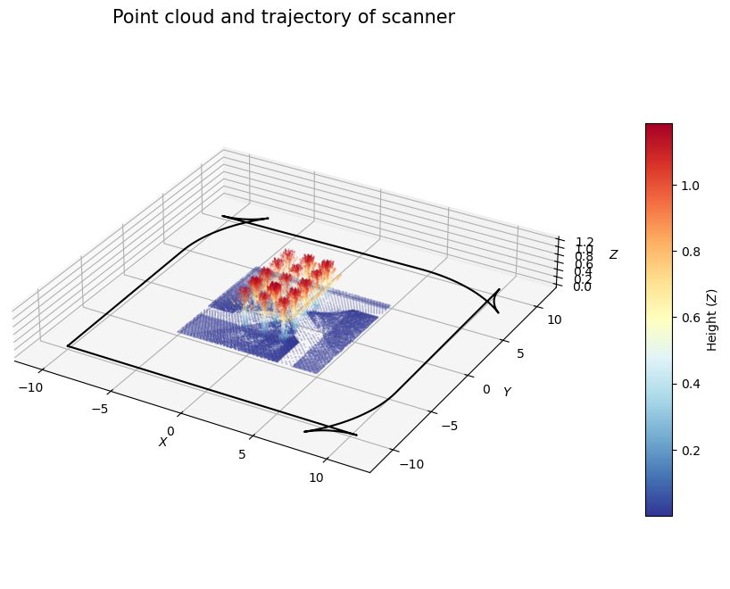
We are using a “RIEGL VZ-400” mounted on a “tractor”. The tractor is a groundvehicle type platform (see platforms.xml), a mobile platform which moves on the ground between the consecutive legs with a constant speed provided by the user. The scannerMount parameter defines the exact position of the scanner and the angle of rotation around the Z- and Y-axis. For the tractor, the scanner is rotated 90° around the Z-axis and -30° around the Y-axis, so that the scene in the center can be capured the best way possible. The ground vehicle tries to mimic real vehicles. It performs “smooth turns” for wide-angle curves. For narrow-angle curves, it first turns, then backs up, then finishes the turn. This can also be seen in the plot later.

scanner = helios.scanner_from_name("riegl_vz_400")
platform = helios.platform_from_name("tractor")

Scanner Settings

# these scanner settings will be shared between all legs
scanner_settings = helios.ScannerSettings(
    pulse_frequency=100_000 * helios.units.Hz,
    scan_frequency=50 * helios.units.Hz,
    scan_angle=20 * helios.units.deg,
    head_rotation="0 deg/s",
    trajectory_time_interval=0.05 * helios.units.s,
)

Survey Route

survey = helios.Survey(scanner=scanner, platform=platform, scene=scene)

waypoints = [[-10, -10, 0], [10, -10, 0], [10, 10, 0], [-10, 10, 0], [-10, -10, 0]]
for x, y, z in waypoints:
    survey.add_leg(x=x, y=y, z=z, speed_m_s=3, scanner_settings=scanner_settings)

Running the survey

points, trajectories = survey.run(
    verbosity=helios.LogVerbosity.VERBOSE, format=helios.OutputFormat.NPY
)

CRS bounding box (by vertices): Min: dvec3(-100.000000, -100.000000, -0.001500), Max: dvec3(100.000000, 100.000000, 1.187800)
Shift: dvec3(0.000000, 0.000000, 0.593150)
# vertices to translate: 3402321
Actual bounding box (by vertices): Min: dvec3(-100.000000, -100.000000, -0.594650), Max: dvec3(100.000000, 100.000000, 0.594650)
Building KD-Grove...
KDTree (num. primitives 1134107) :
        Max. # primitives in leaf: 248
        Min. # primitives in leaf: 1
        Max. depth reached: 41
        KDTree axis-aligned surface area: 80951.4
        Interior nodes: 975880
        Leaf nodes: 747589
        Total tree cost: 6.13429
KDGrove stats:
        Number of trees: 1
        Number of static trees: 1
        Number of dynamic trees: 0
        Statistics (min, max, total, mean, stdev):
                Building time: (1.8560, 1.8560, 1.8560, 1.8560, 0.0000)
                Tree primitives: (1134107, 1134107, 1134107, 1134107.0000, 0.0000)
                Max primitives in leaf: (248, 248, 248, 248.0000, 0.0000)
                Min primitives in leaf: (1, 1, 1, 1.0000, 0.0000)
                Maximum depth: (41, 41, 41, 41.0000, 0.0000)
                Axis-aligned surface area: (80951.4400, 80951.4400, 80951.4400, 80951.4400, 0.0000)
                Number of interior nodes: (975880, 975880, 975880, 975880.0000, 0.0000)
                Number of leaf nodes: (747589, 747589, 747589, 747589.0000, 0.0000)
                Tree cost: (6.1343, 6.1343, 6.1343, 6.1343, 0.0000)

KDG built in 1.857s
Reading Spectral Library...
10 materials found
Warning: material None of primitive 8Triangle (/home/runner/work/helios/helios/example_notebooks/../data/sceneparts/basic/groundplane/groundplane.mtl) has no spectral definition
Number of subsampling rays (riegl_vz400): 19
Simulation: Scanner changed!
Pulse frequency set to 100000
Scan angle set to 20
Applying settings for PolygonMirrorBeamDeflector...
Vertical angle min/max nan/nan degrees
 -- verticalAngleMin not set, using the value of -20 degrees
 -- verticalAngleMax not set, using the value of 20 degrees
SOURCE Leg with serial ID:0 waypoints:
        Origin: (-10, -10, -0.59315)
        Target: (10, -10, -0.59315)
        Next: (10, 10, -0.59315)

It was not possible to determine attitude with a single computation at MovingPlatform::initLegManual
        angle = 3.14159 but it should be below 0.025
        Using iterative computation instead
Iterative mode was used for manual leg initialization because default one failed for MovingPlatform

Starting simulation loop 1 ...
Waypoint reached!
Pulse frequency set to 100000
Scan angle set to 20
Applying settings for PolygonMirrorBeamDeflector...
Vertical angle min/max nan/nan degrees
 -- verticalAngleMin not set, using the value of -20 degrees
 -- verticalAngleMax not set, using the value of 20 degrees
SOURCE Leg with serial ID:1 waypoints:
        Origin: (10, -10, -0.59315)
        Target: (10, 10, -0.59315)
        Next: (-10, 10, -0.59315)

Turn mode 1
Turn mode 2
Waypoint reached!
Pulse frequency set to 100000
Scan angle set to 20
Applying settings for PolygonMirrorBeamDeflector...
Vertical angle min/max nan/nan degrees
 -- verticalAngleMin not set, using the value of -20 degrees
 -- verticalAngleMax not set, using the value of 20 degrees
SOURCE Leg with serial ID:2 waypoints:
        Origin: (10, 10, -0.59315)
        Target: (-10, 10, -0.59315)
        Next: (-10, -10, -0.59315)

Turn mode 1
Turn mode 2
Waypoint reached!
Pulse frequency set to 100000
Scan angle set to 20
Applying settings for PolygonMirrorBeamDeflector...
Vertical angle min/max nan/nan degrees
 -- verticalAngleMin not set, using the value of -20 degrees
 -- verticalAngleMax not set, using the value of 20 degrees
SOURCE Leg with serial ID:3 waypoints:
        Origin: (-10, 10, -0.59315)
        Target: (-10, -10, -0.59315)
        Next: (-10, -10, -0.59315)

Turn mode 1
Turn mode 2
Waypoint reached!
Pulse frequency set to 100000
Scan angle set to 20
Applying settings for PolygonMirrorBeamDeflector...
Vertical angle min/max nan/nan degrees
 -- verticalAngleMin not set, using the value of -20 degrees
 -- verticalAngleMax not set, using the value of 20 degrees
Waypoint reached!
Finishing simulation loop 1 ...
Finished simulation loop 1.
Elapsed simulation steps = 3404024
Elapsed virtual time = 34.0402 sec.
Main thread simulation loop finished in 2.67603 sec.
Waiting for completion of pulse computation tasks...
Pulse computation tasks finished in 2.67604 sec.

Visualizing the results

import matplotlib.pyplot as plt

def extract_by_bb(arr, b_box):
    assert len(b_box) == 6
    x_min, y_min, z_min, x_max, y_max, z_max = b_box
    pos = arr["position"]
    subset = arr[
        (pos[:, 0] > x_min)
        & (pos[:, 0] < x_max)
        & (pos[:, 1] > y_min)
        & (pos[:, 1] < y_max)
        & (pos[:, 2] > z_min)
        & (pos[:, 2] < z_max)
    ]

    return subset

# create scene subset
bbox = [-5, -5, 0, 5, 5, 1.5]

points_sub = extract_by_bb(points, bbox)

fig = plt.figure(figsize=(12, 8))
# 3d plot
ax = fig.add_subplot(projection="3d")

# scatter plot of points
pos = points_sub["position"]
sc = ax.scatter(
    pos[:, 0],
    pos[:, 1],
    pos[:, 2],
    c=pos[:, 2],
    cmap="RdYlBu_r",
    s=0.02,
    label="scene",
)

traj = trajectories["position"]
traj_time = trajectories["gps_time"]
# scatter plot of the trajectory
ax.plot(traj[:, 0], traj[:, 1], traj[:, 2], c="black", label="scanner trajectory")

cax = plt.axes([0.85, 0.2, 0.025, 0.55])
cbar = plt.colorbar(sc, cax=cax)

cbar.set_label("Height ($Z$)")

# Add axis labels.
ax.set_xlabel("$X$")
ax.set_ylabel("$Y$")
ax.set_zlabel("$Z$")

# set equal axes
box = (bbox[3] - bbox[0], bbox[4] - bbox[1], bbox[5] - bbox[2])
ax.set_box_aspect(box)

# Set title.
ax.set_title(label="Point cloud and trajectory of scanner", fontsize=15)

# Display results
plt.show()