ULS Risley Prism Scanner

Notebook: Hannah Weiser & Sina Zumstein, 2023 - 2026

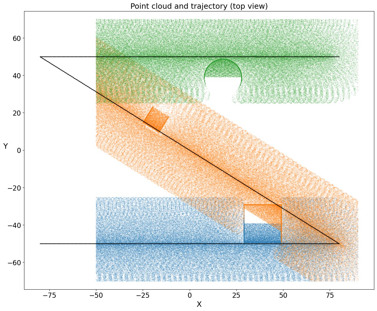
This demo scene showcases a toyblock scene scanned by a risley prism scanner mounted on a UAV.

import helios

Creating the virtual scene

# load objs and apply transformations
groundplane = (
    helios.ScenePart.from_obj("../data/sceneparts/basic/groundplane/groundplane.obj")
    .scale(70)
    .translate([20.0, 0.0, 0.0])
)
cube = helios.ScenePart.from_obj("../data/sceneparts/toyblocks/cube.obj")
cube2 = (
    helios.ScenePart.from_obj("../data/sceneparts/toyblocks/cube.obj")
    .scale(0.5)
    .rotate(axis=(0.0, 0.0, 1.0), angle=45)
    .translate([-45.0, 10.0, 10.0])
)
sphere = helios.ScenePart.from_obj("../data/sceneparts/toyblocks/sphere.obj").scale(0.5)
cylinder = helios.ScenePart.from_obj("../data/sceneparts/toyblocks/cylinder.obj")

# create scene
scene = helios.StaticScene(scene_parts=[groundplane, cube, cube2, sphere, cylinder])

Platform and scanner

scanner = helios.scanner_from_name("livox_mid70")
platform = helios.platform_from_name("copter_linearpath")

The Livox Mid-70 is a scanner with two rotating risley prisms. For this deflector type, the scan pattern is controlled by the rotation speeds of two rotating risley prisms. This design on which the low-cost Livox scanners are based is described in detail in Liu et al. (2022).

For further reading on rotational risley prisms, see Duma & Schitea (2018).

Survey

survey = helios.Survey(scanner=scanner, platform=platform, scene=scene)

scanner_settings = helios.ScannerSettings(
    pulse_frequency=100_000 * helios.units.Hz, trajectory_time_interval=0.05
)

survey.add_leg(x=-80, y=-50, z=35, speed_m_s=5, scanner_settings=scanner_settings)
survey.add_leg(x=80, y=-50, z=35, speed_m_s=5, scanner_settings=scanner_settings)
survey.add_leg(x=-80, y=50, z=35, speed_m_s=5, scanner_settings=scanner_settings)
survey.add_leg(x=80, y=50, z=35, speed_m_s=5, scanner_settings=scanner_settings)

Running the survey

points, trajectories = survey.run(
    verbosity=helios.LogVerbosity.VERBOSE, format=helios.OutputFormat.NPY
)

CRS bounding box (by vertices): Min: dvec3(-50.000000, -70.000000, -0.233912), Max: dvec3(90.000000, 70.000000, 22.012018)
Shift: dvec3(20.000000, 0.000000, 10.889053)
# vertices to translate: 3330
Actual bounding box (by vertices): Min: dvec3(-70.000000, -70.000000, -11.122965), Max: dvec3(70.000000, 70.000000, 11.122965)
Building KD-Grove...
KDTree (num. primitives 1110) :
        Max. # primitives in leaf: 34
        Min. # primitives in leaf: 1
        Max. depth reached: 29
        KDTree axis-aligned surface area: 51657.7
        Interior nodes: 3925
        Leaf nodes: 3474
        Total tree cost: 6.58267
KDGrove stats:
        Number of trees: 1
        Number of static trees: 1
        Number of dynamic trees: 0
        Statistics (min, max, total, mean, stdev):
                Building time: (0.0050, 0.0050, 0.0050, 0.0050, 0.0000)
                Tree primitives: (1110, 1110, 1110, 1110.0000, 0.0000)
                Max primitives in leaf: (34, 34, 34, 34.0000, 0.0000)
                Min primitives in leaf: (1, 1, 1, 1.0000, 0.0000)
                Maximum depth: (29, 29, 29, 29.0000, 0.0000)
                Axis-aligned surface area: (51657.7208, 51657.7208, 51657.7208, 51657.7208, 0.0000)
                Number of interior nodes: (3925, 3925, 3925, 3925.0000, 0.0000)
                Number of leaf nodes: (3474, 3474, 3474, 3474.0000, 0.0000)
                Tree cost: (6.5827, 6.5827, 6.5827, 6.5827, 0.0000)

KDG built in 0.005s
Reading Spectral Library...
10 materials found
Warning: material None of primitive 8Triangle (/home/runner/work/helios/helios/example_notebooks/../data/sceneparts/basic/groundplane/groundplane.mtl) has no spectral definition
Number of subsampling rays (livox_mid-70): 19
Simulation: Scanner changed!
Pulse frequency set to 100000
Scan angle set to 0
It was not possible to determine attitude with a single computation at MovingPlatform::initLegManual
        angle = 3.14159 but it should be below 0.025
        Using iterative computation instead
Iterative mode was used for manual leg initialization because default one failed for MovingPlatform
SOURCE Leg with serial ID:0 waypoints:
        Origin: (-100, -50, 24.1109)
        Target: (60, -50, 24.1109)
        Next: (-100, 50, 24.1109)

Starting simulation loop 1 ...
Waypoint reached!
Pulse frequency set to 100000
Scan angle set to 0
SOURCE Leg with serial ID:1 waypoints:
        Origin: (60, -50, 24.1109)
        Target: (-100, 50, 24.1109)
        Next: (60, 50, 24.1109)

Waypoint reached!
Pulse frequency set to 100000
Scan angle set to 0
It was not possible to determine attitude with a single computation at MovingPlatform::initLegManual
        angle = 1.1172 but it should be below 0.025
        Using iterative computation instead
Iterative mode was used for manual leg initialization because default one failed for MovingPlatform
SOURCE Leg with serial ID:2 waypoints:
        Origin: (-100, 50, 24.1109)
        Target: (60, 50, 24.1109)
        Next: (60, 50, 24.1109)

Waypoint reached!
Pulse frequency set to 100000
Scan angle set to 0
Waypoint reached!
Finishing simulation loop 1 ...
Finished simulation loop 1.
Elapsed simulation steps = 10173598
Elapsed virtual time = 101.736 sec.
Main thread simulation loop finished in 31.4901 sec.
Waiting for completion of pulse computation tasks...
Pulse computation tasks finished in 31.4901 sec.

Visualizing the results

import matplotlib.pyplot as plt

fig, ax = plt.subplots(figsize=(15, 12))
strip_1 = points[points["point_source_id"] == 0]["position"]
strip_2 = points[points["point_source_id"] == 1]["position"]
strip_3 = points[points["point_source_id"] == 2]["position"]
traj = trajectories["position"]

# view from above, colored by strip, including trajectory - show only every 20th measurement
ax.scatter(
    strip_1[::20, 0], strip_1[::20, 1], s=0.05, alpha=0.6
)  # select X and Y coordinates
ax.scatter(strip_2[::20, 0], strip_2[::20, 1], s=0.05, alpha=0.6)
ax.scatter(strip_3[::20, 0], strip_3[::20, 1], s=0.05, alpha=0.6)
ax.scatter(traj[:, 0], traj[:, 1], s=0.5, color="black")
ax.tick_params(labelsize=16)
ax.set_xlabel("X", fontsize=18)
ax.set_ylabel("Y", fontsize=18, rotation=0)

ax.set_title("Point cloud and trajectory (top view)", fontsize=18)

plt.axis("equal")
plt.show()