TLS voxelized point cloud
Notebook: Hannah Weiser, 2026
This demo shows how to load a point cloud as scene part, which is then converted to a voxel model by HELIOS++. The example point cloud is a sphere, and we will scan it with terrestrial laser scanning (TLS).
Imports
[1]:
import helios
import numpy as np
import matplotlib.pyplot as plt
Creating the virtual scene
This scene consists of a simple ground plane loaded from an OBJ file and a point cloud of a sphere which is loaded from an XYZ file. HELIOS++ is transforming this point cloud into a voxel model, which is then scanned. The size of the voxels is determined by the value provided to the parameter voxel_size, here 1.0 meters.
Furthermore, we tell HELIOS++ to estimate normals for each voxel by setting estimate_normals to 1. This means that not the normal vector of the outer surface of each voxel cube is used, but instead the normal vector computed from the points within the voxel. These normal vectors determine the incidence angle of the beam, which in return influences the intensity that is computed for the generated return.
[2]:
# load objs and create transformations
groundplane = helios.ScenePart.from_obj(
    "../data/sceneparts/basic/groundplane/groundplane.obj"
).scale(100)
sphere = helios.ScenePart.from_xyz(
    "../data/sceneparts/pointclouds/sphere_dens25000.xyz",
    voxel_size=1.0,
    separator=" ",
    estimate_normals=1,
).translate([0.0, 0.0, 10.0])

# create scene
scene = helios.StaticScene(scene_parts=[groundplane, sphere])
Platform and scanner
HELIOS++ comes with a wide range of pre-defined scanners and platforms, which we can import and instantiate from the scanner and platforms submodules by their ID. We use the tripod platform (a simple static platform with the scanner mounted at a height of 1.5 m), and the RIEGL VZ-400 TLS.
[3]:
scanner = helios.scanner_from_name("riegl_vz_400")
platform = helios.platform_from_name("tripod")
Scan positions and scanner settings
[4]:
survey = helios.Survey(scanner=scanner, platform=platform, scene=scene)
# first scan position
survey.add_leg(
    x=40.0,
    y=-10.0,
    z=0.0,
    force_on_ground=True,  # this works because of the specification in the groundplane.mtl file,
    pulse_frequency=100_000 * helios.units.Hz,
    scan_frequency=120 * helios.units.Hz,
    min_vertical_angle=-40 * helios.units.deg,
    max_vertical_angle=60 * helios.units.deg,
    rotation_start_angle=250 * helios.units.deg,
    rotation_stop_angle=380 * helios.units.deg,
    head_rotation="10 deg/s",
)
Running the survey
[5]:
points, _ = survey.run(
    verbosity=helios.LogVerbosity.VERBOSE, format=helios.OutputFormat.NPY
)
CRS bounding box (by vertices): Min: dvec3(-100.000000, -100.000000, 0.000000), Max: dvec3(100.000000, 100.000000, 54.029834)
Shift: dvec3(0.000000, 0.000000, 27.014917)
# vertices to translate: 6206
Actual bounding box (by vertices): Min: dvec3(-100.000000, -100.000000, -27.014917), Max: dvec3(100.000000, 100.000000, 27.014917)
Building KD-Grove...
KDTree (num. primitives 6202) :
        Max. # primitives in leaf: 16
        Min. # primitives in leaf: 1
        Max. depth reached: 32
        KDTree axis-aligned surface area: 122824
        Interior nodes: 35068
        Leaf nodes: 34249
        Total tree cost: 5.03407
KDGrove stats:
        Number of trees: 1
        Number of static trees: 1
        Number of dynamic trees: 0
        Statistics (min, max, total, mean, stdev):
                Building time: (0.0530, 0.0530, 0.0530, 0.0530, 0.0000)
                Tree primitives: (6202, 6202, 6202, 6202.0000, 0.0000)
                Max primitives in leaf: (16, 16, 16, 16.0000, 0.0000)
                Min primitives in leaf: (1, 1, 1, 1.0000, 0.0000)
                Maximum depth: (32, 32, 32, 32.0000, 0.0000)
                Axis-aligned surface area: (122823.8670, 122823.8670, 122823.8670, 122823.8670, 0.0000)
                Number of interior nodes: (35068, 35068, 35068, 35068.0000, 0.0000)
                Number of leaf nodes: (34249, 34249, 34249, 34249.0000, 0.0000)
                Tree cost: (5.0341, 5.0341, 5.0341, 5.0341, 0.0000)

KDG built in 0.053s
Reading Spectral Library...
10 materials found
Warning: material None of primitive 8Triangle (/home/runner/work/helios/helios/example_notebooks/../data/sceneparts/basic/groundplane/groundplane.mtl) has no spectral definition
Number of subsampling rays (riegl_vz400): 19
Simulation: Scanner changed!
Pulse frequency set to 100000
Scan angle set to 120
Applying settings for PolygonMirrorBeamDeflector...
Vertical angle min/max -40/60 degrees
Starting simulation loop 1 ...
Finishing simulation loop 1 ...
Finished simulation loop 1.
Elapsed simulation steps = 1300002
Elapsed virtual time = 13 sec.
Main thread simulation loop finished in 1.73233 sec.
Waiting for completion of pulse computation tasks...
Pulse computation tasks finished in 1.73234 sec.
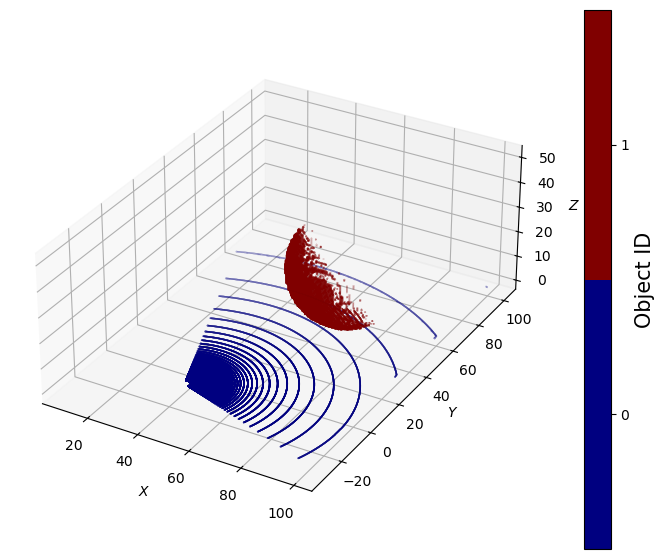
Visualizing the result
Finally, let’s visualize the simulated points using matplotlib.
[6]:
coords = points["position"]
object_id = points["hit_object_id"]

# Matplotlib figures.
fig = plt.figure(figsize=(9, 7))

# settings for a discrete colorbar
N = 2
cmap = plt.get_cmap("jet", N)

# Scatter plot of the point cloud (coloured by hitObjectId).
ax = fig.add_subplot(projection="3d")
sc = ax.scatter(
    coords[:, 0],
    coords[:, 1],
    coords[:, 2],
    c=object_id,
    cmap=cmap,
    s=0.02,
    label="scene",
)

# Add axis labels.
ax.set_xlabel("$X$")
ax.set_ylabel("$Y$")
ax.set_zlabel("$Z$")

# set equal axes
box = (np.ptp(coords[:, 0]), np.ptp(coords[:, 1]), np.ptp(coords[:, 2]))
ax.set_box_aspect(box)

cbar = plt.colorbar(sc, ticks=[1 / 4, 3 / 4])

cbar.set_label("Object ID", fontsize=15)
cbar.ax.set_yticklabels(["0", "1"])

# Display results
plt.show()
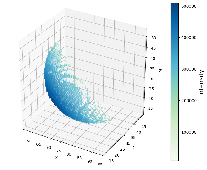
[7]:
# select only points with object ID = 1
sphere_idx = object_id == 1

# get coords and intensities
sphere_coords = coords[sphere_idx, :]
sphere_intensities = points["intensity"][sphere_idx]

# Matplotlib figures.
fig = plt.figure(figsize=(9, 7))

# Scatter plot of only the sphere point cloud (coloured by Intensity).
ax = fig.add_subplot(projection="3d")
sc = ax.scatter(
    sphere_coords[:, 0],
    sphere_coords[:, 1],
    sphere_coords[:, 2],
    c=sphere_intensities,
    cmap="GnBu",
    s=0.1,
    label="scene",
)

# Add axis labels.
ax.set_xlabel("$X$")
ax.set_ylabel("$Y$")
ax.set_zlabel("$Z$")

# set equal axes
box = (
    np.ptp(sphere_coords[:, 0]),
    np.ptp(sphere_coords[:, 1]),
    np.ptp(sphere_coords[:, 2]),
)
ax.set_box_aspect(box)

cbar = plt.colorbar(sc)

cbar.set_label("Intensity", fontsize=15)

plt.show()
[ ]: