ALS over a DTM (Heidelberg)

Notebook creator: Hannah Weiser, 2026

This demo uses a digital terrain model (DTM) of Heidelberg, Germany, which will be scanned by airborne laser scanning (ALS).

import helios
import matplotlib.pyplot as plt
import matplotlib.colors as mcolors

Creating the virtual scene

# load geotiff
dtm = helios.ScenePart.from_tiff("../data/sceneparts/tiff/dem_hd.tif")
# scene
scene = helios.StaticScene(scene_parts=[dtm])

Platform and Scanner

scanner = helios.scanner_from_name("leica_als50_ii")
platform = helios.platform_from_name("sr22")

Scanner and platform settings

# these scanner settings will be shared between all legs
scanner_settings = helios.ScannerSettings(
    pulse_frequency=60_000 * helios.units.Hz,
    scan_frequency=50 * helios.units.Hz,
    scan_angle=60 * helios.units.deg,
    trajectory_time_interval=0.05 * helios.units.s,
)
# Q: How to change detector settings (like maximum range) in a survey???

z = 1500.0  # m
speed = 150  # m/s

Survey Route

survey = helios.Survey(scanner=scanner, platform=platform, scene=scene)

waypoints = [[474500, 5474500], [490000, 5474500], [474500, 5473500], [490000, 5473500]]
for x, y in waypoints:
    survey.add_leg(x=x, y=y, z=z, speed_m_s=speed, scanner_settings=scanner_settings)

Running the survey

points, trajectories = survey.run(
    verbosity=helios.LogVerbosity.VERBOSE, format=helios.OutputFormat.NPY
)

Scene::doForceGround could not compute nothing because there was no ground scene part available
CRS bounding box (by vertices): Min: dvec3(465335.125829, 5464987.890296, 34.000000), Max: dvec3(491335.125829, 5482787.890296, 581.000000)
Shift: dvec3(478335.125829, 5473887.890296, 307.500000)
# vertices to translate: 4442880
Actual bounding box (by vertices): Min: dvec3(-13000.000000, -8900.000000, -273.500000), Max: dvec3(13000.000000, 8900.000000, 273.500000)
Building KD-Grove...
KDTree (num. primitives 1480960) :
        Max. # primitives in leaf: 300
        Min. # primitives in leaf: 1
        Max. depth reached: 37
        KDTree axis-aligned surface area: 9.73517e+08
        Interior nodes: 2261571
        Leaf nodes: 1972154
        Total tree cost: 12.6756
KDGrove stats:
        Number of trees: 1
        Number of static trees: 1
        Number of dynamic trees: 0
        Statistics (min, max, total, mean, stdev):
                Building time: (3.3070, 3.3070, 3.3070, 3.3070, 0.0000)
                Tree primitives: (1480960, 1480960, 1480960, 1480960.0000, 0.0000)
                Max primitives in leaf: (300, 300, 300, 300.0000, 0.0000)
                Min primitives in leaf: (1, 1, 1, 1.0000, 0.0000)
                Maximum depth: (37, 37, 37, 37.0000, 0.0000)
                Axis-aligned surface area: (973517200.0000, 973517200.0000, 973517200.0000, 973517200.0000, 0.0000)
                Number of interior nodes: (2261571, 2261571, 2261571, 2261571.0000, 0.0000)
                Number of leaf nodes: (1972154, 1972154, 1972154, 1972154.0000, 0.0000)
                Tree cost: (12.6756, 12.6756, 12.6756, 12.6756, 0.0000)

KDG built in 3.309s
Reading Spectral Library...
10 materials found
Warning: material default of primitive 8Triangle () has no spectral definition
Number of subsampling rays (leica_als50-ii): 19
Simulation: Scanner changed!
Pulse frequency set to 60000
Scan angle set to 60 degrees.
Scan frequency set to 50 Hz.
It was not possible to determine attitude with a single computation at MovingPlatform::initLegManual
        angle = 3.14159 but it should be below 0.025
        Using iterative computation instead
Iterative mode was used for manual leg initialization because default one failed for MovingPlatform
SOURCE Leg with serial ID:0 waypoints:
        Origin: (-3835.13, 612.11, 1192.5)
        Target: (11664.9, 612.11, 1192.5)
        Next: (-3835.13, -387.89, 1192.5)

Starting simulation loop 1 ...
Waypoint reached!
Pulse frequency set to 60000
Scan angle set to 60 degrees.
Scan frequency set to 50 Hz.
It was not possible to determine attitude with a single computation at MovingPlatform::initLegManual
        angle = 0.128854 but it should be below 0.025
        Using iterative computation instead
Iterative mode was used for manual leg initialization because default one failed for MovingPlatform
SOURCE Leg with serial ID:1 waypoints:
        Origin: (11664.9, 612.11, 1192.5)
        Target: (-3835.13, -387.89, 1192.5)
        Next: (11664.9, -387.89, 1192.5)

Waypoint reached!
Pulse frequency set to 60000
Scan angle set to 60 degrees.
Scan frequency set to 50 Hz.
SOURCE Leg with serial ID:2 waypoints:
        Origin: (-3835.13, -387.89, 1192.5)
        Target: (11664.9, -387.89, 1192.5)
        Next: (11664.9, -387.89, 1192.5)

Waypoint reached!
Pulse frequency set to 60000
Scan angle set to 60 degrees.
Scan frequency set to 50 Hz.
Waypoint reached!
Finishing simulation loop 1 ...
Finished simulation loop 1.
Elapsed simulation steps = 18612895
Elapsed virtual time = 310.215 sec.
Main thread simulation loop finished in 208.717 sec.
Waiting for completion of pulse computation tasks...
Pulse computation tasks finished in 208.717 sec.

Visualizing the results

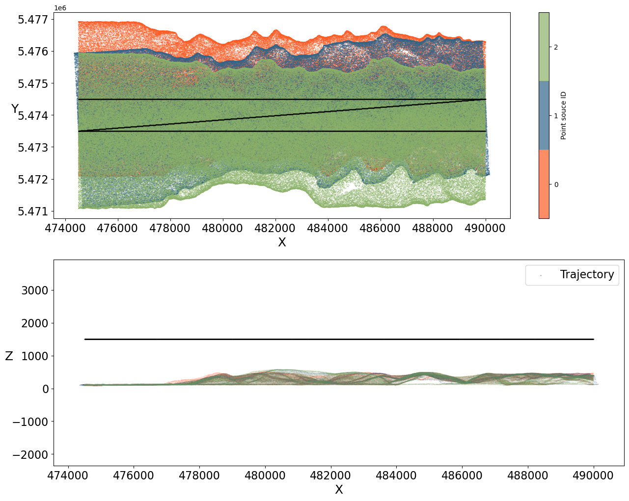
Now we can display a couple of 2D plots of the simulated point cloud. We create two plots - one from above and one from the side - showing the point cloud colored by flight strip and the trajectory.

# two subplots
fig, (ax1, ax2) = plt.subplots(2, figsize=(15, 12))
pos = points["position"]
traj = trajectories["position"]

N = 3
colors = ["#FE5D26", "#33658A", "#8CB369"]
rgba_colors = [mcolors.to_rgba(c) for c in colors]
cmap = mcolors.ListedColormap(
    rgba_colors, name="custom"
)  # discrete colormap with 3 colors

# view from above, colored by strip, including trajectory - for faster display, show only every 25th measurement
sc = ax1.scatter(
    pos[::25, 0],
    pos[::25, 1],
    s=0.1,
    alpha=0.7,
    c=points["point_source_id"][::25],
    cmap=cmap,
    vmin=-0.5,
    vmax=N - 0.5,
)
ax1.scatter(traj[:, 0], traj[:, 1], s=0.1, label="Trajectory", color="black")
ax1.tick_params(labelsize=16)
ax1.set_xlabel("X", fontsize=18)
ax1.set_ylabel("Y", fontsize=18, rotation=0)

plt.colorbar(sc, ticks=[0, 1, 2], label="Point souce ID")

# use only every 50th measurement for better display
ax2.scatter(
    pos[::50, 0],
    pos[::50, 2],
    alpha=0.05,
    s=0.1,
    c=points["point_source_id"][::50],
    cmap=cmap,
    vmin=-0.5,
    vmax=N - 0.5,
)  # select X and Z coordinates
ax2.scatter(traj[:, 0], traj[:, 2], s=0.05, label="Trajectory", color="black")
ax2.tick_params(labelsize=16)
ax2.set_xlabel("X", fontsize=18)
ax2.set_ylabel("Z", fontsize=18, rotation=0)
ax2.legend(fontsize=16)

plt.axis("equal")
plt.show()

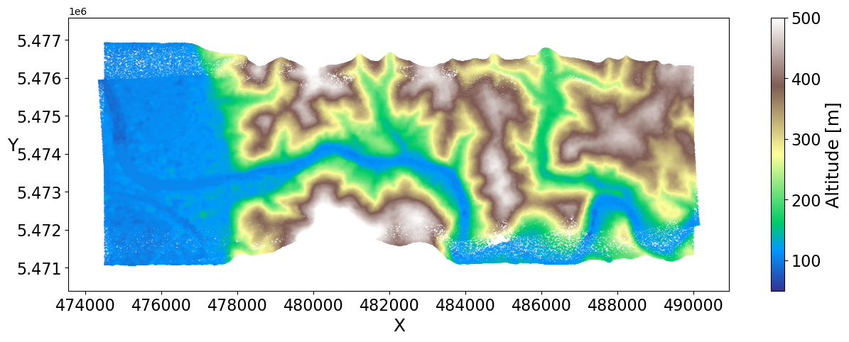
Let’s create another plot from above which is colored by altitude.

# view from above - colored by altitude
fig, ax = plt.subplots(figsize=(15, 5))

# select X and y coordinates
plot1 = ax.scatter(
    pos[::20, 0],
    pos[::20, 1],
    s=0.1,
    c=pos[::20, 2],
    cmap="terrain",
    vmin=50,
    vmax=500,
)

plt.axis("equal")
ax.tick_params(labelsize=16)
plt.xlabel("X", fontsize=18)
plt.ylabel("Y", fontsize=18, rotation=0)

cbar = plt.colorbar(plot1)
cbar.ax.tick_params(labelsize=16)
cbar.set_label("Altitude [m]", fontsize=18)
plt.show()

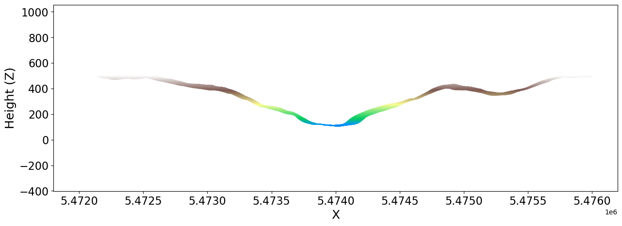
Finally, plot only a section of the point cloud to get a profile of the Neckar valley in Heidelberg.

# Section in direction of Y
xmin, ymin, xmax, ymax = [480000, 5472000, 480100, 5476000]

section = pos[
    (pos[:, 0] > xmin) & (pos[:, 0] < xmax) & (pos[:, 1] > ymin) & (pos[:, 1] < ymax)
]

fig = plt.figure(figsize=(15, 5))
ax = fig.add_subplot()

ax.scatter(
    section[:, 1],
    section[:, 2],
    c=section[:, 2],
    cmap="terrain",
    s=0.01,
    vmin=50,
    vmax=500,
)
ax.tick_params(labelsize=16)

plt.xlabel("X", fontsize=18)
plt.ylabel("Height (Z)", fontsize=18, rotation=90)
plt.axis("equal")
plt.show()