Trajectory interpolation
Notebook: Lukas Winiwarter, 2023 and Hannah Weiser, 2026
In this demo, we present how an existing or external trajectory can be used to model platform location and attitude in a HELIOS++ simulation.
[1]:
from pathlib import Path
from IPython.display import Code
import helios
from helios.platforms import Platform, load_traj_csv
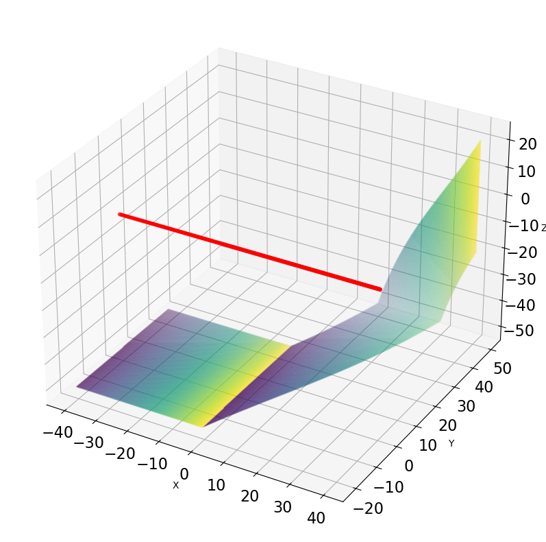
In this example, we simulate an airborne laser scanner acquisition flying inside of a box of 100 m side length. This allows us to see the full point pattern.
We set the platform to interpolated, and define a trajectory file in the tag. This is provided by a filename and a column order. By setting syncGPSTime, we ensure that the output point cloud is in the same time system as the input trajectory.
[2]:
box = helios.ScenePart.from_obj("../data/sceneparts/basic/box/box100.obj")
scene = helios.StaticScene(scene_parts=[box])
[3]:
scanner = helios.scanner_from_name("riegl_lms_q560")
trajectory = load_traj_csv(
    csv="../data/trajectories/flyandrotate.trj",
    tIndex=0,
    xIndex=4,
    yIndex=5,
    zIndex=6,
    rollIndex=1,
    pitchIndex=2,
    yawIndex=3,
)

platform = Platform.load_interpolate_platform(
    trajectory,
    "data/platforms.xml",
    "sr22",
    sync_gps_time=True,
    interpolation_method="ARINC 705",
)  # default interpolation_mode
[4]:
trajectory
[4]:
array([( 0. , 0.        , 0., 0.        ,   0., -40., 0.),
       ( 2.5, 0.        , 0., 0.        ,   0.,   0., 0.),
       ( 5. , 1.57079633, 0., 0.        ,   0.,  40., 0.),
       ( 5. , 0.        , 0., 1.57079633, -40.,   0., 0.),
       ( 7.5, 0.        , 0., 1.57079633,   0.,   0., 0.),
       (10. , 1.57079633, 0., 1.57079633,  40.,   0., 0.)],
      dtype=[('t', '<f8'), ('roll', '<f8'), ('pitch', '<f8'), ('yaw', '<f8'), ('x', '<f8'), ('y', '<f8'), ('z', '<f8')])
The contents of the trajectory file are simple: For the first 2.5 seconds, we move from (0, -40, 0) to (0, 0, 0), with a constant attitude of (0,0,0) (roll, pitch, yaw). In the next 2.5 seconds, we continue to move to (0, 40, 0), but rotate (roll) until we have an attitude of (90, 0, 0). HELIOS++ linearly interpolates between these values.
The second half of the file shows a movement from (-40, 0, 0) to (40, 0, 0). Note how, for the interpolated platform, the yaw angle has to be set explicitely, in this case to 90 degrees (i.e., east). Apart from these changes, the roll rotation is the same as in the first half of the file.
[5]:
scanner_settings = helios.ScannerSettings(
    is_active=True,
    pulse_frequency=180_000 * helios.units.Hz,
    scan_frequency=100 * helios.units.Hz,
    trajectory_time_interval=0.01,
)
trajectory_settings1 = helios.TrajectorySettings(start_time=0, end_time=5)
trajectory_settings2 = helios.TrajectorySettings(start_time=5, end_time=10)

survey = helios.Survey(scanner=scanner, platform=platform, scene=scene)
survey.add_leg(
    scanner_settings=scanner_settings, trajectory_settings=trajectory_settings1
)
survey.add_leg(
    scanner_settings=scanner_settings, trajectory_settings=trajectory_settings2
)
[6]:
Code(open("../data/trajectories/flyandrotate.trj").read())
[6]:
#TIME_COLUMN: 0
#HEADER: "t", "roll", "pitch", "yaw", "x", "y", "z"
0, 0, 0, 0, 0, -40, 0
2.5, 0, 0, 0, 0, 0, 0
5, 90, 0, 0, 0, 40, 0
5, 0, 0, 90, -40, 0, 0
7.5, 0, 0, 90, 0, 0, 0
10, 90, 0, 90, 40, 0, 0
Running the survey
[7]:
points, traj = survey.run(verbosity=helios.LogVerbosity.VERBOSE)
Scene::doForceGround could not compute nothing because there was no ground scene part available
CRS bounding box (by vertices): Min: dvec3(-50.000000, -50.000000, -50.000000), Max: dvec3(50.000000, 50.000000, 50.000000)
Shift: dvec3(0.000000, 0.000000, 0.000000)
# vertices to translate: 36
Actual bounding box (by vertices): Min: dvec3(-50.000000, -50.000000, -50.000000), Max: dvec3(50.000000, 50.000000, 50.000000)
Building KD-Grove...
KDTree (num. primitives 12) :
        Max. # primitives in leaf: 6
        Min. # primitives in leaf: 4
        Max. depth reached: 13
        KDTree axis-aligned surface area: 60000
        Interior nodes: 76
        Leaf nodes: 77
        Total tree cost: 9.03226
KDGrove stats:
        Number of trees: 1
        Number of static trees: 1
        Number of dynamic trees: 0
        Statistics (min, max, total, mean, stdev):
                Building time: (0.0010, 0.0010, 0.0010, 0.0010, 0.0000)
                Tree primitives: (12, 12, 12, 12.0000, 0.0000)
                Max primitives in leaf: (6, 6, 6, 6.0000, 0.0000)
                Min primitives in leaf: (4, 4, 4, 4.0000, 0.0000)
                Maximum depth: (13, 13, 13, 13.0000, 0.0000)
                Axis-aligned surface area: (60000.0000, 60000.0000, 60000.0000, 60000.0000, 0.0000)
                Number of interior nodes: (76, 76, 76, 76.0000, 0.0000)
                Number of leaf nodes: (77, 77, 77, 77.0000, 0.0000)
                Tree cost: (9.0323, 9.0323, 9.0323, 9.0323, 0.0000)

KDG built in 0.001s
Reading Spectral Library...
10 materials found
Warning: material Material of primitive 8Triangle (/home/runner/work/helios/helios/example_notebooks/../data/sceneparts/basic/box/box100.mtl) has no spectral definition
Number of subsampling rays (riegl_lms-q560): 19
Simulation: Scanner changed!
Pulse frequency set to 180000
Scan angle set to 45
Applying settings for PolygonMirrorBeamDeflector...
Vertical angle min/max nan/nan degrees
 -- verticalAngleMin not set, using the value of -22.5 degrees
 -- verticalAngleMax not set, using the value of 22.5 degrees
SOURCE Leg with serial ID:0 waypoints:
        Origin: (0, -40, 0)
        Target: (-40, 0, 0)
        Next: (-40, 0, 0)
Starting simulation loop 1 ...
Pulse frequency set to 180000
Scan angle set to 45
Applying settings for PolygonMirrorBeamDeflector...
Vertical angle min/max nan/nan degrees
 -- verticalAngleMin not set, using the value of -22.5 degrees
 -- verticalAngleMax not set, using the value of 22.5 degrees
STOP Leg with serial ID:0 waypoints:
        Origin: (-40, 0, 0)
        Target: (-40, 0, 0)
        Next: (40, 0, 0)

Pulse frequency set to 180000
Scan angle set to 45
Applying settings for PolygonMirrorBeamDeflector...
Vertical angle min/max nan/nan degrees
 -- verticalAngleMin not set, using the value of -22.5 degrees
 -- verticalAngleMax not set, using the value of 22.5 degrees
SOURCE Leg with serial ID:1 waypoints:
        Origin: (-40, 0, 0)
        Target: (40, 0, 0)
        Next: (40, 0, 0)

Pulse frequency set to 180000
Scan angle set to 45
Applying settings for PolygonMirrorBeamDeflector...
Vertical angle min/max nan/nan degrees
 -- verticalAngleMin not set, using the value of -22.5 degrees
 -- verticalAngleMax not set, using the value of 22.5 degrees
Finishing simulation loop 1 ...
Finished simulation loop 1.
Elapsed simulation steps = 1800004
Elapsed virtual time = 10 sec.
Main thread simulation loop finished in 4.19702 sec.
Waiting for completion of pulse computation tasks...
Pulse computation tasks finished in 4.19703 sec.
Visualizing the result
[8]:
import matplotlib.pyplot as plt

fig = plt.figure(figsize=(15, 10))
ax = fig.add_subplot(projection="3d")

pc1 = points[points["gps_time"] <= 2.5]
pc2 = points[(points["gps_time"] > 2.5) & (points["gps_time"] < 5)]

trj = traj[traj["gps_time"] < 5]["position"]

ax.scatter(
    pc1["position"][:, 0],
    pc1["position"][:, 1],
    pc1["position"][:, 2],
    s=0.001,
    c=pc1["gps_time"],
)
ax.scatter(
    pc2["position"][:, 0],
    pc2["position"][:, 1],
    pc2["position"][:, 2],
    s=0.001,
    c=pc2["gps_time"],
)
ax.scatter(trj[:, 0], trj[:, 1], trj[:, 2], s=10, c="red")
ax.set_xlabel("X")
ax.set_ylabel("Y")
ax.set_zlabel("Z")

ax.tick_params(labelsize=16)
plt.show()
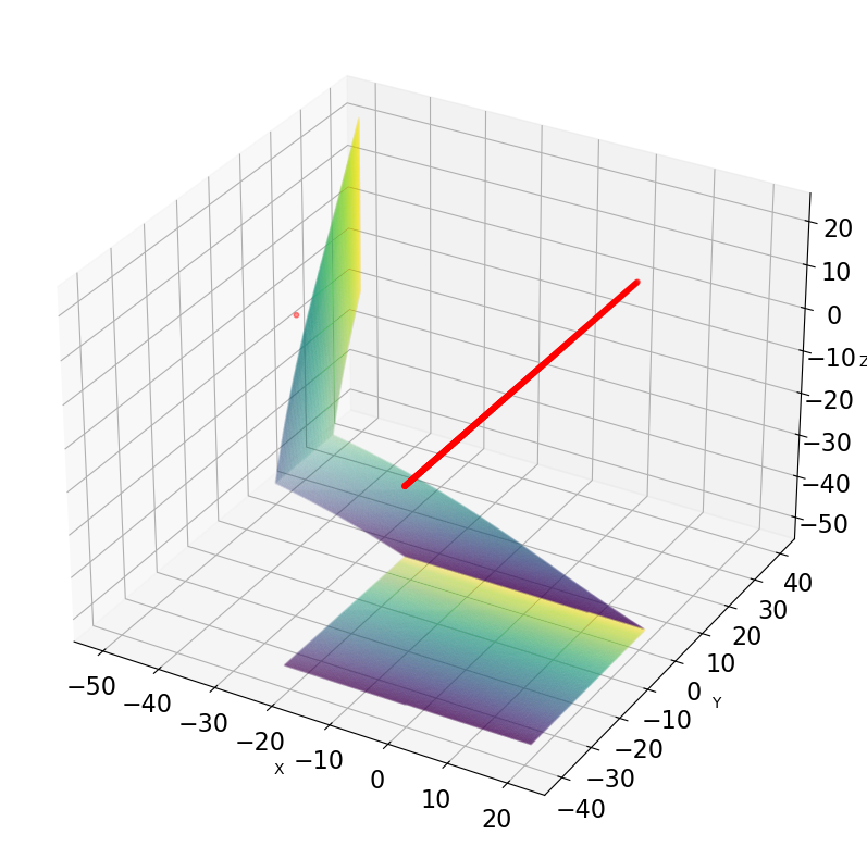
[9]:
import matplotlib.pyplot as plt

fig = plt.figure(figsize=(15, 10))
ax = fig.add_subplot(projection="3d")

pc1 = points[(points["gps_time"] >= 5) & (points["gps_time"] < 7.5)]
pc2 = points[points["gps_time"] > 7.5]

trj = traj[traj["gps_time"] >= 5]["position"]

ax.scatter(
    pc1["position"][:, 0],
    pc1["position"][:, 1],
    pc1["position"][:, 2],
    s=0.001,
    c=pc1["gps_time"],
)
ax.scatter(
    pc2["position"][:, 0],
    pc2["position"][:, 1],
    pc2["position"][:, 2],
    s=0.001,
    c=pc2["gps_time"],
)
ax.scatter(trj[:, 0], trj[:, 1], trj[:, 2], s=10, c="red")
ax.set_xlabel("X")
ax.set_ylabel("Y")
ax.set_zlabel("Z")

ax.tick_params(labelsize=16)
plt.show()