MLS toyblocks
Notebook creator: Hannah Weiser, 2026
This demo uses a toy scene, which will be scanned by ground-based mobile laser scanning (MLS).
[1]:
import helios
import numpy as np
import matplotlib.pyplot as plt
Creating the virtual scene
[2]:
# load objs and apply transformations
groundplane = (
    helios.ScenePart.from_obj("../data/sceneparts/basic/groundplane/groundplane.obj")
    .scale(70)
    .translate([20.0, 0.0, 0.0])
)
cube = helios.ScenePart.from_obj("../data/sceneparts/toyblocks/cube.obj")
cube2 = (
    helios.ScenePart.from_obj("../data/sceneparts/toyblocks/cube.obj")
    .scale(0.5)
    .rotate(axis=(0.0, 0.0, 1.0), angle=45)
    .translate([-45.0, 10.0, 10.0])
)
sphere = helios.ScenePart.from_obj("../data/sceneparts/toyblocks/sphere.obj").scale(0.5)
cylinder = helios.ScenePart.from_obj("../data/sceneparts/toyblocks/cylinder.obj")

# create scene
scene = helios.StaticScene(scene_parts=[groundplane, cube, cube2, sphere, cylinder])
Platform and Scanner
[3]:
scanner = helios.scanner_from_name("riegl_vux_1ha22")
platform = helios.platform_from_name("vmq_1ha_car")
Scanner Settings
[4]:
# these scanner settings will be shared between all legs
scanner_settings = helios.ScannerSettings(
    pulse_frequency=100_000 * helios.units.Hz,
    scan_frequency=50 * helios.units.Hz,
    scan_angle=180 * helios.units.deg,
    head_rotation="0 deg/s",
    trajectory_time_interval=0.05 * helios.units.s,
)
Survey Route
[5]:
survey = helios.Survey(scanner=scanner, platform=platform, scene=scene)
[6]:
waypoints = [
    [-30, 65.0, 0],
    [-25.0, -30.0, 0],
    [1.0, -30.0, 0],
    [31.0, 0.0, 0],
    [73.5, 0.0, 0],
]
for x, y, z in waypoints:
    survey.add_leg(x=x, y=y, z=z, speed_m_s=20.0, scanner_settings=scanner_settings)
Running the survey
[7]:
points, trajectories = survey.run(
    verbosity=helios.LogVerbosity.VERBOSE, format=helios.OutputFormat.NPY
)
CRS bounding box (by vertices): Min: dvec3(-50.000000, -70.000000, -0.233912), Max: dvec3(90.000000, 70.000000, 22.012018)
Shift: dvec3(20.000000, 0.000000, 10.889053)
# vertices to translate: 3330
Actual bounding box (by vertices): Min: dvec3(-70.000000, -70.000000, -11.122965), Max: dvec3(70.000000, 70.000000, 11.122965)
Building KD-Grove...
KDTree (num. primitives 1110) :
        Max. # primitives in leaf: 34
        Min. # primitives in leaf: 1
        Max. depth reached: 29
        KDTree axis-aligned surface area: 51657.7
        Interior nodes: 3941
        Leaf nodes: 3486
        Total tree cost: 6.58266
KDGrove stats:
        Number of trees: 1
        Number of static trees: 1
        Number of dynamic trees: 0
        Statistics (min, max, total, mean, stdev):
                Building time: (0.0050, 0.0050, 0.0050, 0.0050, 0.0000)
                Tree primitives: (1110, 1110, 1110, 1110.0000, 0.0000)
                Max primitives in leaf: (34, 34, 34, 34.0000, 0.0000)
                Min primitives in leaf: (1, 1, 1, 1.0000, 0.0000)
                Maximum depth: (29, 29, 29, 29.0000, 0.0000)
                Axis-aligned surface area: (51657.7208, 51657.7208, 51657.7208, 51657.7208, 0.0000)
                Number of interior nodes: (3941, 3941, 3941, 3941.0000, 0.0000)
                Number of leaf nodes: (3486, 3486, 3486, 3486.0000, 0.0000)
                Tree cost: (6.5827, 6.5827, 6.5827, 6.5827, 0.0000)

KDG built in 0.005s
Reading Spectral Library...
10 materials found
Warning: material None of primitive 8Triangle (/home/runner/work/helios/helios/example_notebooks/../data/sceneparts/basic/groundplane/groundplane.mtl) has no spectral definition
Number of subsampling rays (riegl_vux-1ha22): 19
Simulation: Scanner changed!
WARNING: Specified pulse frequency is not supported by this device. We'll set it nevertheless.

Pulse frequency set to 100000
Scan angle set to 180
Applying settings for PolygonMirrorBeamDeflector...
Vertical angle min/max nan/nan degrees
 -- verticalAngleMin not set, using the value of -180 degrees
 -- verticalAngleMax not set, using the value of 180 degrees
It was not possible to determine attitude with a single computation at MovingPlatform::initLegManual
        angle = 0.105166 but it should be below 0.025
        Using iterative computation instead
Iterative mode was used for manual leg initialization because default one failed for MovingPlatform
SOURCE Leg with serial ID:0 waypoints:
        Origin: (-50, 65, -10.8891)
        Target: (-45, -30, -10.8891)
        Next: (-19, -30, -10.8891)
Starting simulation loop 1 ...
Waypoint reached!
WARNING: Specified pulse frequency is not supported by this device. We'll set it nevertheless.

Pulse frequency set to 100000
Scan angle set to 180
Applying settings for PolygonMirrorBeamDeflector...
Vertical angle min/max nan/nan degrees
 -- verticalAngleMin not set, using the value of -180 degrees
 -- verticalAngleMax not set, using the value of 180 degrees
SOURCE Leg with serial ID:1 waypoints:
        Origin: (-45, -30, -10.8891)
        Target: (-19, -30, -10.8891)
        Next: (11, 0, -10.8891)

Waypoint reached!
WARNING: Specified pulse frequency is not supported by this device. We'll set it nevertheless.

Pulse frequency set to 100000
Scan angle set to 180
Applying settings for PolygonMirrorBeamDeflector...
Vertical angle min/max nan/nan degrees
 -- verticalAngleMin not set, using the value of -180 degrees
 -- verticalAngleMax not set, using the value of 180 degrees
SOURCE Leg with serial ID:2 waypoints:
        Origin: (-19, -30, -10.8891)
        Target: (11, 0, -10.8891)
        Next: (53.5, 0, -10.8891)

Waypoint reached!
WARNING: Specified pulse frequency is not supported by this device. We'll set it nevertheless.

Pulse frequency set to 100000
Scan angle set to 180
Applying settings for PolygonMirrorBeamDeflector...
Vertical angle min/max nan/nan degrees
 -- verticalAngleMin not set, using the value of -180 degrees
 -- verticalAngleMax not set, using the value of 180 degrees
It was not possible to determine attitude with a single computation at MovingPlatform::initLegManual
        angle = 1.57079 but it should be below 0.025
        Using iterative computation instead
Iterative mode was used for manual leg initialization because default one failed for MovingPlatform
SOURCE Leg with serial ID:3 waypoints:
        Origin: (11, 0, -10.8891)
        Target: (53.5, 0, -10.8891)
        Next: (53.5, 0, -10.8891)

Waypoint reached!
WARNING: Specified pulse frequency is not supported by this device. We'll set it nevertheless.

Pulse frequency set to 100000
Scan angle set to 180
Applying settings for PolygonMirrorBeamDeflector...
Vertical angle min/max nan/nan degrees
 -- verticalAngleMin not set, using the value of -180 degrees
 -- verticalAngleMax not set, using the value of 180 degrees
Waypoint reached!
Finishing simulation loop 1 ...
Finished simulation loop 1.
Elapsed simulation steps = 1030296
Elapsed virtual time = 10.303 sec.
Main thread simulation loop finished in 3.35311 sec.
Waiting for completion of pulse computation tasks...
Pulse computation tasks finished in 3.35311 sec.
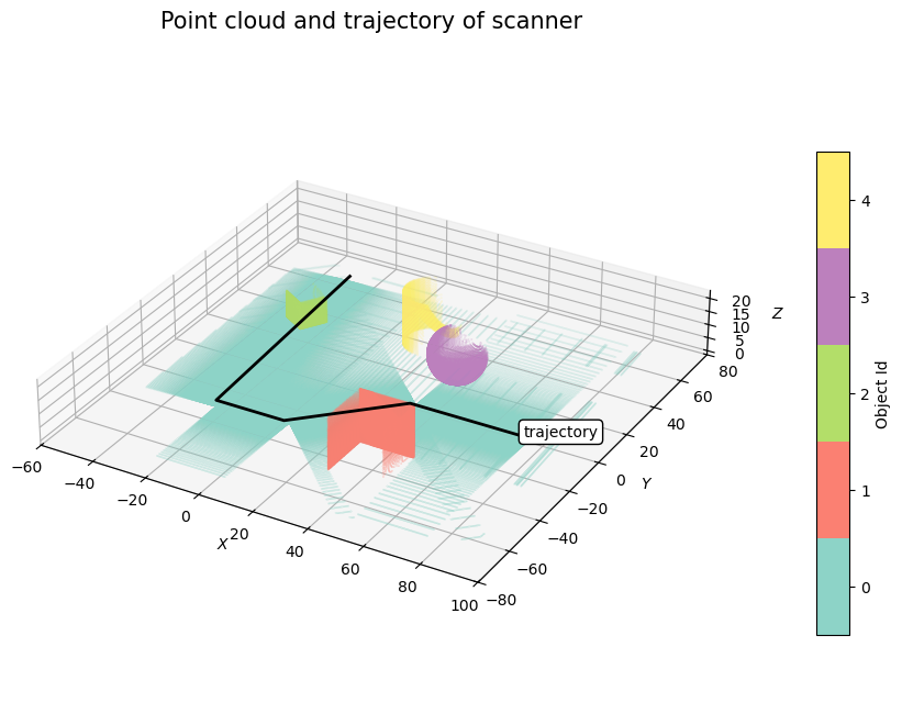
Visualizing the results
Color by Object ID
[8]:
fig = plt.figure(figsize=(12, 8))
# 3d plot
ax = fig.add_subplot(projection="3d", computed_zorder=False)

# settings for a discrete colorbar
N = 5
cmap = plt.get_cmap("Set3", N)

# scatter plot of points
pos = points["position"]
sc = ax.scatter(
    pos[:, 0],
    pos[:, 1],
    pos[:, 2],
    c=points["hit_object_id"],
    cmap=cmap,
    s=0.02,
    zorder=1,
    vmin=-0.5,
    vmax=4.5,
)

traj = trajectories["position"]
# Plot of trajectory
ax.plot(traj[:, 0], traj[:, 1], traj[:, 2], c="black", linewidth=2, zorder=2)

cax = plt.axes([0.85, 0.2, 0.025, 0.55])
cbar = plt.colorbar(sc, cax=cax, ticks=[0, 1, 2, 3, 4])
cbar.ax.set_yticklabels(["0", "1", "2", "3", "4"])
cbar.set_label("Object Id")

# Add axis labels.
ax.set_xlabel("$X$")
ax.set_ylabel("$Y$")
ax.set_zlabel("$Z$")

# set equal axes
box = (np.ptp(pos[:, 0]), np.ptp(pos[:, 1]), np.ptp(pos[:, 2]))
ax.set_box_aspect(box)

# Set title.
ax.set_title(label="Point cloud and trajectory of scanner", fontsize=15)
ax.text(
    traj[-1, 0],
    traj[-1, 1],
    traj[-1, 2],
    "trajectory",
    bbox=dict(boxstyle="round", fc="w", ec="k"),
    size="10",
)

# Display results
plt.show()
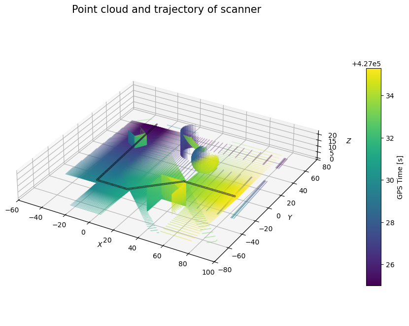
Color by GPS Time
[9]:
# Matplotlib figure
fig = plt.figure(figsize=(12, 8))
# Axes3d axis onto mpl figure.
ax = fig.add_subplot(projection="3d", computed_zorder=False)

# Scatter plot of points (coloured by GPS time)
time = points["gps_time"]
sc_pc = ax.scatter(pos[:, 0], pos[:, 1], pos[:, 2], c=time, s=0.02, zorder=1)

# Plot of trajectory.
sc_traj = ax.scatter(
    traj[:, 0],
    traj[:, 1],
    traj[:, 2],
    c=trajectories["gps_time"],
    s=5,
    zorder=2,
    lw=0.5,
)
sc_traj.set_edgecolor("black")

cax = plt.axes([0.85, 0.2, 0.025, 0.55])
cbar = plt.colorbar(sc_pc, cax=cax)
cbar.set_label("GPS Time [s]")

# Add axis labels.
ax.set_xlabel("$X$")
ax.set_ylabel("$Y$")
ax.set_zlabel("$Z$")

# set equal axes
ax.set_box_aspect(box)

# Set title.
ax.set_title(label="Point cloud and trajectory of scanner", fontsize=15)

# Display results
plt.show()
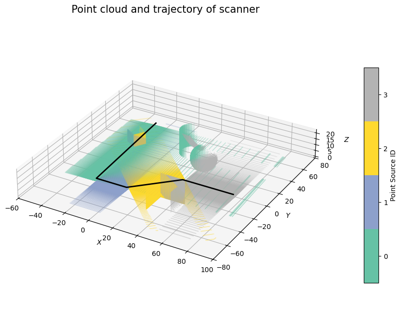
Color by point source ID (strip ID)
[10]:
# Matplotlib figure
fig = plt.figure(figsize=(12, 8))
# Axes3d axis onto mpl figure.
ax = fig.add_subplot(projection="3d", computed_zorder=False)

# settings for a discrete colorbar
N = 4
cmap = plt.get_cmap("Set2", N)

# Scatter plot of points (coloured by point source ID)
sc_pc = ax.scatter(
    pos[:, 0],
    pos[:, 1],
    pos[:, 2],
    c=points["point_source_id"],
    s=0.02,
    zorder=1,
    cmap=cmap,
    vmin=-0.5,
    vmax=3.5,
)

# Plot of trajectory
ax.plot(traj[:, 0], traj[:, 1], traj[:, 2], c="black", linewidth=2, zorder=2)

cax = plt.axes([0.85, 0.2, 0.025, 0.55])
cbar = plt.colorbar(sc_pc, cax=cax, ticks=[0, 1, 2, 3])
cbar.ax.set_yticklabels(["0", "1", "2", "3"])
cbar.set_label("Point Source ID")

# Add axis labels.
ax.set_xlabel("$X$")
ax.set_ylabel("$Y$")
ax.set_zlabel("$Z$")

# set equal axes
ax.set_box_aspect(box)

# Set title.
ax.set_title(label="Point cloud and trajectory of scanner", fontsize=15)

# Display results
plt.show()