ALS with Multi-Channel Risley Scanner

Notebook: Hannah Weiser, 2026

This demo shows the simulation using a risley based scanner with three sensors, the Livox Mid-100.

import helios
import numpy as np
import matplotlib.pyplot as plt

Scanner and platform

As scanner, we use the Livox Mid-100, which has three LiDAR sensors (Mid-40s) with overlapping fields of view.

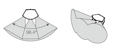
Multi-channel laser scanner Livox Mid-100. Source: Livox datasheet.

platform = helios.platform_from_name("sr22")
scanner = helios.scanner_from_name("livox_mid100")

Scene

As scene, we use the simple toyblocks scene.

groundplane = helios.ScenePart.from_obj(
    "../data/sceneparts/basic/groundplane/groundplane.obj"
).scale(100.0)
cube = helios.ScenePart.from_obj("../data/sceneparts/toyblocks/cube.obj")
# ToDo: Write issue to support translating scene parts on ground
cube2 = (
    helios.ScenePart.from_obj("../data/sceneparts/toyblocks/cube.obj")
    .rotate(axis=[0, 0, 1], angle=45.0 * helios.units.deg)
    .scale(0.5)
    .translate([-45.0, 10.0, 10.0])
)

scene = helios.StaticScene([groundplane, cube, cube2])

Survey

survey = helios.Survey(scene=scene, platform=platform, scanner=scanner)
z = 100.0
speed = 30  # m/s

survey.add_leg(x=-30.0, y=-50.0, z=z, speed_m_s=speed)
survey.add_leg(x=70.0, y=-50.0, z=z, speed_m_s=speed, is_active=False)
survey.add_leg(x=70.0, y=50.0, z=z, speed_m_s=speed)
survey.add_leg(x=-30.0, y=50.0, z=z, speed_m_s=speed, is_active=False)

Running the survey

pc, traj = survey.run()

coords = pc["position"]
traj_coords = traj["position"]

Visualizing the results

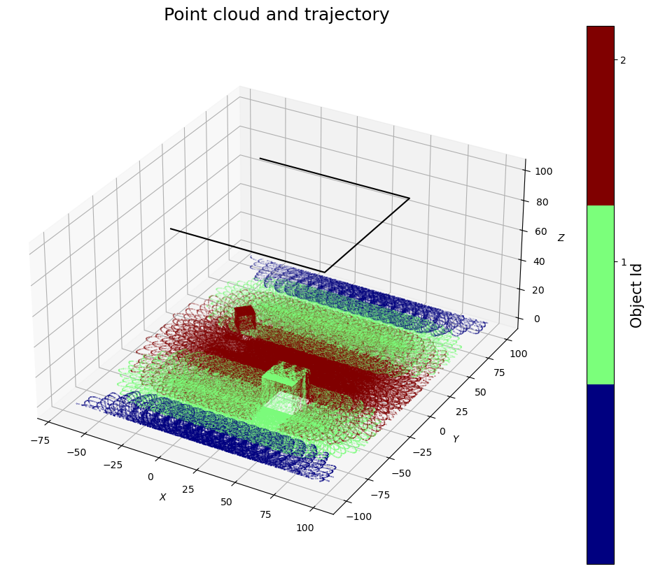
1) Full point cloud coloured by channel ID

We plot the point cloud coloured by channel ID, i.e., the points of the three sensors of the Livox Mid-100 are shown in different colours.

# matplotlib figure
fig = plt.figure(figsize=(15, 10))

# settings for a discrete colorbar
N = 3
cmap = plt.get_cmap("jet", N)

# Scatter plot of (coloured by hitObjectId).
ax = fig.add_subplot(1, 1, 1, projection="3d")
sc = ax.scatter(
    coords[::10, 0],
    coords[::10, 1],
    coords[::10, 2],
    c=pc["channel_id"][::10],
    cmap=cmap,
    s=0.02,
)
# Plot of trajectory.
ax.plot(traj_coords[:, 0], traj_coords[:, 1], traj_coords[:, 2], c="black")

# Add axis labels.
ax.set_xlabel("$X$")
ax.set_ylabel("$Y$")
ax.set_zlabel("$Z$")

# set equal axes in x and y, exaggerated z by a factor of 5
box = (np.ptp(coords[:, 0]), np.ptp(coords[:, 1]), np.ptp(coords[:, 2]) * 5)
ax.set_box_aspect(box)

# Set title
ax.set_title(label="Point cloud and trajectory", fontsize=18)

# colorbar with discrete ticks
tick_locs = (np.arange(1, N + 1) + 0.5) * (N) / (N + 1)
cbar = plt.colorbar(sc, ticks=tick_locs)

cbar.set_label("Object Id", fontsize=15)
tick_labels = [str(i) for i in range(1, N + 1)]
cbar.ax.set_yticklabels(tick_labels)

# Display results
plt.show()

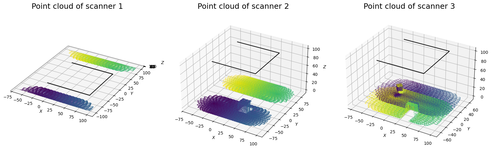
2) Subplots split by channel ID and coloured by GPS time

Below, we split the point cloud by channel ID and plot the points of each channel in a separate subplot. The points are coloured by GPS time,.

# we load the output of each scanner and strip seperately
channel1 = pc[pc["channel_id"] == 0]
channel2 = pc[pc["channel_id"] == 1]
channel3 = pc[pc["channel_id"] == 2]

# Matplotlib figures.
fig = plt.figure(figsize=(20, 12))

for i, coords in enumerate([channel1, channel2, channel3]):

    # Scatter plot of points from respective scanner (coloured by GpsTime).
    ax = fig.add_subplot(1, 3, i + 1, projection="3d")
    sc = ax.scatter(
        coords["position"][::10, 0],
        coords["position"][::10, 1],
        coords["position"][::10, 2],
        c=coords["gps_time"][::10],
        cmap="viridis",
        s=0.02,
    )

    # Plot of trajectory.
    ax.plot(traj_coords[:, 0], traj_coords[:, 1], traj_coords[:, 2], c="black")

    # Add axis labels.
    ax.set_xlabel("$X$")
    ax.set_ylabel("$Y$")
    ax.set_zlabel("$Z$")

    # set equal axes in x and y, exaggerated z by a factor of 5
    box = (
        np.ptp(coords["position"][:, 0]),
        np.ptp(coords["position"][:, 1]),
        np.ptp(coords["position"][:, 2]) * 5,
    )
    ax.set_box_aspect(box)

    # Set title.
    ax.set_title(label=f"Point cloud of scanner {i+1}", fontsize=18)

# Display results
plt.show()