ALS over a DTM with constant height above ground (Heidelberg)
Notebook creator: Hannah Weiser, 2026
This demo uses a digital terrain model (DTM) of Heidelberg, Germany, which will be scanned by airborne laser scanning (ALS), maintaining a constant height above ground using interpolated trajectories.
[1]:
from pathlib import Path
import helios
import numpy as np
import matplotlib.pyplot as plt
import matplotlib.colors as mcolors
import math
from scipy.interpolate import CubicSpline, make_interp_spline
import rasterio as rio
from helios.platforms import Platform, load_traj_csv
[2]:
def interpolate_waypoints(t, x, y, time_step, b_spline_degree=3):
    """Interpolates waypoints to create a smooth trajectory using cubic splines."""

    # Generate new time points
    new_t = np.arange(t[0], t[-1] + time_step, time_step)
    fx = make_interp_spline(t, x, b_spline_degree)
    fy = make_interp_spline(t, y, b_spline_degree)

    # Interpolate x and y
    new_x = fx(new_t)
    new_y = fy(new_t)

    return new_t, new_x, new_y


def compute_yaw_angles(x, y):
    yaw_angles = []
    for i in range(len(x) - 1):
        dx = x[i + 1] - x[i]
        dy = y[i + 1] - y[i]
        yaw = np.arctan2(dx, dy)
        # Normalize yaw to be in the range [0, 2π)
        if yaw < 0:
            yaw += 2 * np.pi
        # Append the yaw angle
        yaw_angles.append(yaw)

    # Append the last yaw angle
    yaw_angles.append(yaw_angles[-1])

    return np.array(yaw_angles)


def follow_height_above_ground(x, y, height_agl, dtm_file):
    coords = np.array([x, y]).T
    with rio.open(dtm_file) as src:
        z_vals = [z[0] + height_agl for z in src.sample(coords)]

    return np.array(z_vals)
Creating the virtual scene
[3]:
# load geotiff
dtm_file = "../data/sceneparts/tiff/dem_hd.tif"
dtm = helios.ScenePart.from_tiff(dtm_file)
# scene
scene = helios.StaticScene(scene_parts=[dtm])
Scanner
[4]:
scanner = helios.scanner_from_name("leica_als50")
Survey Route
[5]:
waypoints = np.array(
    [
        [477280.4, 5472582.6],
        [480531.0, 5472590.9],
        [480553.9, 5473285.3],
        [477304.6, 5473277.0],
        [477313.5, 5473863.9],
        [480567.7, 5473888.6],
    ]
)

# compute time assuming constant speed
speed_m_s = 250
distances_between_waypoints = np.linalg.norm(np.diff(waypoints, axis=0), axis=1)
times = [0]
for distance in distances_between_waypoints:
    times.append(times[-1] + distance / speed_m_s)
[6]:
# interpolate waypoints to create a trajectory
time_step = 0.2  # s
height_agl = 1000  # m
t, x, y = interpolate_waypoints(
    times, waypoints[:, 0], waypoints[:, 1], time_step=time_step, b_spline_degree=1
)

z = follow_height_above_ground(x, y, height_agl, dtm_file)

roll = np.zeros(len(x))  # Assuming roll is zero for simplicity
pitch = np.zeros(len(x))  # Assuming pitch is zero for simplicity
yaw = compute_yaw_angles(x, y)
waypoints_final = np.zeros(
    len(x),
    dtype={
        "names": ("t", "roll", "pitch", "yaw", "x", "y", "z"),
        "formats": ("f8", "f8", "f8", "f8", "f8", "f8", "f8"),
    },
)
waypoints_final["x"] = x
waypoints_final["y"] = y
waypoints_final["z"] = z
waypoints_final["t"] = t
waypoints_final["roll"] = roll
waypoints_final["pitch"] = pitch
waypoints_final["yaw"] = yaw
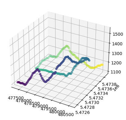
[7]:
# plot trajectory
ax = plt.figure().add_subplot(projection="3d")
ax.scatter(
    waypoints_final["x"],
    waypoints_final["y"],
    waypoints_final["z"],
    "ro-",
    label="Trajectory",
    c=waypoints_final["t"],
)
plt.show()
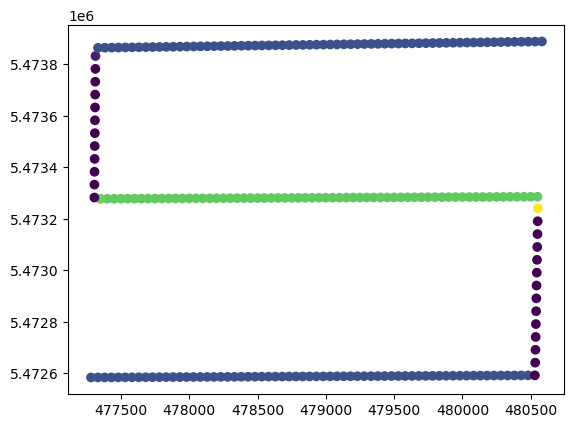
[8]:
# plot from above coloured by yaw
plt.scatter(waypoints_final["x"], waypoints_final["y"], c=waypoints_final["yaw"])
plt.show()
Platfrom and scanner settings
[9]:
platform = Platform.load_interpolate_platform(
    trajectory=waypoints_final,
    platform_file="data/platforms.xml",
    platform_id="sr22",
    interpolation_method="CANONICAL",
    sync_gps_time=True,
)
[10]:
scanner_settings = helios.ScannerSettings(
    pulse_frequency=83_000 * helios.units.Hz,
    scan_frequency=50 * helios.units.Hz,
    scan_angle=30 * helios.units.deg,
    head_rotation="0 deg/s",
    trajectory_time_interval=0.06 * helios.units.s,
)
[11]:
survey = helios.Survey(scanner=scanner, platform=platform, scene=scene)
for i in range(len(times) - 1):
    print(f"Adding leg {i} from {times[i]} to {times[i+1]}")
    trajectory_settings_leg = helios.platforms.TrajectorySettings(
        start_time=times[i], end_time=times[i + 1], teleport_to_start=True
    )
    survey.add_leg(
        scanner_settings=scanner_settings, trajectory_settings=trajectory_settings_leg
    )
Adding leg 0 from 0 to 13.00244238595187
Adding leg 1 from 13.00244238595187 to 15.78155237297786
Adding leg 2 from 15.78155237297786 to 28.778794775887977
Adding leg 3 from 28.778794775887977 to 31.126664687106867
Adding leg 4 from 31.126664687106867 to 44.14383963714886
Running the survey
[12]:
points, trajectory = survey.run(verbosity=helios.LogVerbosity.VERBOSE)
Scene::doForceGround could not compute nothing because there was no ground scene part available
CRS bounding box (by vertices): Min: dvec3(465335.125829, 5464987.890296, 34.000000), Max: dvec3(491335.125829, 5482787.890296, 581.000000)
Shift: dvec3(478335.125829, 5473887.890296, 307.500000)
# vertices to translate: 4442880
Actual bounding box (by vertices): Min: dvec3(-13000.000000, -8900.000000, -273.500000), Max: dvec3(13000.000000, 8900.000000, 273.500000)
Building KD-Grove...
KDTree (num. primitives 1480960) :
        Max. # primitives in leaf: 300
        Min. # primitives in leaf: 1
        Max. depth reached: 37
        KDTree axis-aligned surface area: 9.73517e+08
        Interior nodes: 2262578
        Leaf nodes: 1973178
        Total tree cost: 12.6757
KDGrove stats:
        Number of trees: 1
        Number of static trees: 1
        Number of dynamic trees: 0
        Statistics (min, max, total, mean, stdev):
                Building time: (3.4060, 3.4060, 3.4060, 3.4060, 0.0000)
                Tree primitives: (1480960, 1480960, 1480960, 1480960.0000, 0.0000)
                Max primitives in leaf: (300, 300, 300, 300.0000, 0.0000)
                Min primitives in leaf: (1, 1, 1, 1.0000, 0.0000)
                Maximum depth: (37, 37, 37, 37.0000, 0.0000)
                Axis-aligned surface area: (973517200.0000, 973517200.0000, 973517200.0000, 973517200.0000, 0.0000)
                Number of interior nodes: (2262578, 2262578, 2262578, 2262578.0000, 0.0000)
                Number of leaf nodes: (1973178, 1973178, 1973178, 1973178.0000, 0.0000)
                Tree cost: (12.6757, 12.6757, 12.6757, 12.6757, 0.0000)

KDG built in 3.407s
Reading Spectral Library...
10 materials found
Warning: material default of primitive 8Triangle () has no spectral definition
Number of subsampling rays (leica_als50): 19
Simulation: Scanner changed!
Pulse frequency set to 83000
Scan angle set to 30 degrees.
Scan frequency set to 50 Hz.
TELEPORT Leg with serial ID:0 waypoints:
        Origin: (-1054.73, -1305.29, 811.5)
        Target: (-1054.73, -1305.29, 811.5)
        Next: (2195.29, -1296.39, 1188.37)
Starting simulation loop 1 ...
Pulse frequency set to 83000
Scan angle set to 30 degrees.
Scan frequency set to 50 Hz.
SOURCE Leg with serial ID:0 waypoints:
        Origin: (-1054.73, -1305.29, 811.5)
        Target: (2195.29, -1296.39, 1188.37)
        Next: (2195.29, -1296.39, 1188.37)

Pulse frequency set to 83000
Scan angle set to 30 degrees.
Scan frequency set to 50 Hz.
STOP Leg with serial ID:0 waypoints:
        Origin: (2195.29, -1296.39, 1188.37)
        Target: (2195.29, -1296.39, 1188.37)
        Next: (2195.29, -1296.39, 1188.37)

Pulse frequency set to 83000
Scan angle set to 30 degrees.
Scan frequency set to 50 Hz.
TELEPORT Leg with serial ID:1 waypoints:
        Origin: (2195.29, -1296.39, 1188.37)
        Target: (2195.29, -1296.39, 1188.37)
        Next: (2214.45, -606.785, 1050.53)

Pulse frequency set to 83000
Scan angle set to 30 degrees.
Scan frequency set to 50 Hz.
SOURCE Leg with serial ID:1 waypoints:
        Origin: (2195.29, -1296.39, 1188.37)
        Target: (2214.45, -606.785, 1050.53)
        Next: (2214.45, -606.785, 1050.53)

Pulse frequency set to 83000
Scan angle set to 30 degrees.
Scan frequency set to 50 Hz.
STOP Leg with serial ID:1 waypoints:
        Origin: (2214.45, -606.785, 1050.53)
        Target: (2214.45, -606.785, 1050.53)
        Next: (2214.45, -606.785, 1050.53)

Pulse frequency set to 83000
Scan angle set to 30 degrees.
Scan frequency set to 50 Hz.
TELEPORT Leg with serial ID:2 waypoints:
        Origin: (2214.45, -606.785, 1050.53)
        Target: (2214.45, -606.785, 1050.53)
        Next: (-1025.71, -606.14, 799.606)

Pulse frequency set to 83000
Scan angle set to 30 degrees.
Scan frequency set to 50 Hz.
SOURCE Leg with serial ID:2 waypoints:
        Origin: (2214.45, -606.785, 1050.53)
        Target: (-1025.71, -606.14, 799.606)
        Next: (-1025.71, -606.14, 799.606)

Pulse frequency set to 83000
Scan angle set to 30 degrees.
Scan frequency set to 50 Hz.
STOP Leg with serial ID:2 waypoints:
        Origin: (-1025.71, -606.14, 799.606)
        Target: (-1025.71, -606.14, 799.606)
        Next: (-1025.71, -606.14, 799.606)

Pulse frequency set to 83000
Scan angle set to 30 degrees.
Scan frequency set to 50 Hz.
TELEPORT Leg with serial ID:3 waypoints:
        Origin: (-1025.71, -606.14, 799.606)
        Target: (-1025.71, -606.14, 799.606)
        Next: (-1010.19, -35.5121, 812.3)

Pulse frequency set to 83000
Scan angle set to 30 degrees.
Scan frequency set to 50 Hz.
SOURCE Leg with serial ID:3 waypoints:
        Origin: (-1025.71, -606.14, 799.606)
        Target: (-1010.19, -35.5121, 812.3)
        Next: (-1010.19, -35.5121, 812.3)

Pulse frequency set to 83000
Scan angle set to 30 degrees.
Scan frequency set to 50 Hz.
STOP Leg with serial ID:3 waypoints:
        Origin: (-1010.19, -35.5121, 812.3)
        Target: (-1010.19, -35.5121, 812.3)
        Next: (-1010.19, -35.5121, 812.3)

Pulse frequency set to 83000
Scan angle set to 30 degrees.
Scan frequency set to 50 Hz.
TELEPORT Leg with serial ID:4 waypoints:
        Origin: (-1010.19, -35.5121, 812.3)
        Target: (-1010.19, -35.5121, 812.3)
        Next: (2232.57, 0.709704, 871.658)

Pulse frequency set to 83000
Scan angle set to 30 degrees.
Scan frequency set to 50 Hz.
SOURCE Leg with serial ID:4 waypoints:
        Origin: (-1010.19, -35.5121, 812.3)
        Target: (2232.57, 0.709704, 871.658)
        Next: (2232.57, 0.709704, 871.658)

Pulse frequency set to 83000
Scan angle set to 30 degrees.
Scan frequency set to 50 Hz.
Finishing simulation loop 1 ...
Finished simulation loop 1.
Elapsed simulation steps = 3663952
Elapsed virtual time = 44.144 sec.
Main thread simulation loop finished in 36.8913 sec.
Waiting for completion of pulse computation tasks...
Pulse computation tasks finished in 36.8913 sec.
[13]:
points["position"]
[13]:
array([[4.77281819e+05, 5.47298743e+06, 1.25185534e+02],
       [4.77281818e+05, 5.47298583e+06, 1.25291485e+02],
       [4.77281817e+05, 5.47298428e+06, 1.25269764e+02],
       ...,
       [4.80569309e+05, 5.47410991e+06, 1.16515569e+02],
       [4.80569324e+05, 5.47411145e+06, 1.16307795e+02],
       [4.80569575e+05, 5.47413786e+06, 1.12314020e+02]],
      shape=(3663937, 3))
[14]:
trajectory["position"]
[14]:
array([[4.77280403e+05, 5.47258260e+06, 1.11900018e+03],
       [4.77280406e+05, 5.47258260e+06, 1.11900036e+03],
       [4.77295406e+05, 5.47258264e+06, 1.11990036e+03],
       ...,
       [4.80523420e+05, 5.47388826e+06, 1.17600139e+03],
       [4.80538419e+05, 5.47388838e+06, 1.17740069e+03],
       [4.80553419e+05, 5.47388849e+06, 1.17830069e+03]], shape=(739, 3))
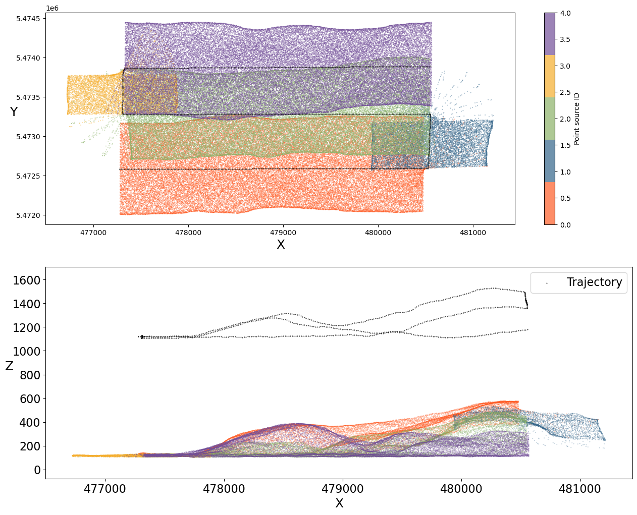
Visualizing the results
Now we can display a couple of 2D plots of the simulated point cloud.
[15]:
# two subplots
fig, (ax1, ax2) = plt.subplots(2, figsize=(15, 12))
pos = points["position"]
traj = trajectory["position"]

N = 5
colors = ["#FE5D26", "#33658A", "#8CB369", "#F6AE2D", "#724E99"]  # 5 distinct colors
rgba_colors = [mcolors.to_rgba(c) for c in colors]
cmap = mcolors.ListedColormap(
    rgba_colors, name="custom"
)  # discrete colormap with 3 colors

# view from above, colored by strip, including trajectory - for faster display, show only every 25th measurement
sc = ax1.scatter(
    pos[::25, 0],
    pos[::25, 1],
    s=0.1,
    alpha=0.7,
    c=points["point_source_id"][::25],
    cmap=cmap,
    # vmin=-0.5, vmax=N - 0.5
)
ax1.scatter(traj[:, 0], traj[:, 1], s=0.2, label="Trajectory", color="black")
ax1.set_xlabel("X", fontsize=18)
ax1.set_ylabel("Y", fontsize=18, rotation=0)

plt.colorbar(sc, label="Point source ID")

# use only every 50th measurement for better display
ax2.scatter(
    pos[::50, 0],
    pos[::50, 2],
    alpha=0.7,
    s=0.05,
    c=points["point_source_id"][::50],
    cmap=cmap,
    # vmin=-0.5, vmax=N - 0.5
)  # select X and Z coordinates
ax2.scatter(traj[:, 0], traj[:, 2], s=0.2, label="Trajectory", color="black")
ax2.tick_params(labelsize=16)
ax2.set_xlabel("X", fontsize=18)
ax2.set_ylabel("Z", fontsize=18, rotation=0)
ax2.legend(fontsize=16)

plt.axis("equal")
plt.show()
[ ]: